Text data

Text data#

Text data is one of the most widely used forms of data in the digital age. It encompasses everything from simple written words to complex documents and entire libraries of knowledge. Text is the primary data type in natural language processing (NLP). Text data are usually organized as a collection of documents, e.g., books, social media posts, emails, log files, etc.

There are several ways how to convert a document to numeric format.

Bag of words#

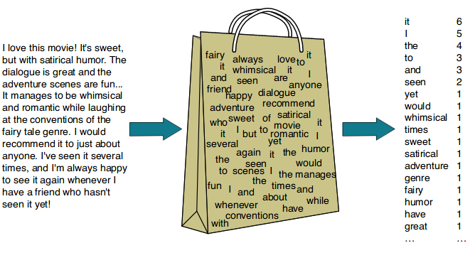
https://miro.medium.com/v2/resize:fit:661/1*sX2Y1Y9Au0hCJzj9qQBV5g.png

The bag of words (BoW) model represents text as a collection of words, disregarding grammar and word order but keeping multiplicity. To obtain a numeric representation of a document one needs:

tokenize the text into words;
create a vocabulary of all unique words in the corpus;
represent each document as a vector where each dimension corresponds to a word in the vocabulary, and the value is the frequency of that word in the document.

Toy example#

Consider the following sentences.

“I love machine learning”
“Machine learning is fun”
“I love programming”
“Programming is fun”
“Machine learning is important”
“Math for fun”
“Learning math is important for machine learning”

Count matrix#

We have \(10\) unique words in this corpus. Now just count all the words in each sentence:

#Sentence	I	love	machine	learning	is	fun	programming	important	math	for
1	1	1	1	1	0	0	0	0	0	0
2	0	0	1	1	1	1	0	0	0	0
3	1	1	0	0	0	0	1	0	0	0
4	0	0	0	0	1	1	1	0	0	0
5	0	0	1	1	1	0	0	1	0	0
6	0	0	0	0	0	1	0	0	1	1
7	0	0	1	2	1	0	0	1	1	1

Disadvantages of BoW#

The bag of words model is a simple method for text representation, but it has several drawbacks:

Loss of semantic meaning. The BoW model ignores the order and context of words. For example, “dog bites man” and “man bites dog” would have the same representation, even though their meanings are quite different.
High dimensionality and sparsity. The dimensionality of the vector space grows with the size of the vocabulary. Also, most documents use only a small subset of the total vocabulary, leading to sparse vectors.
Lack of focus on important words. All words are treated with equal importance, regardless of their relevance to the document’s content
Difficulty in handling out-of-vocabulary words. Any word not present in the vocabulary will be ignored or cause an issue during vectorization.

TF-IDF#

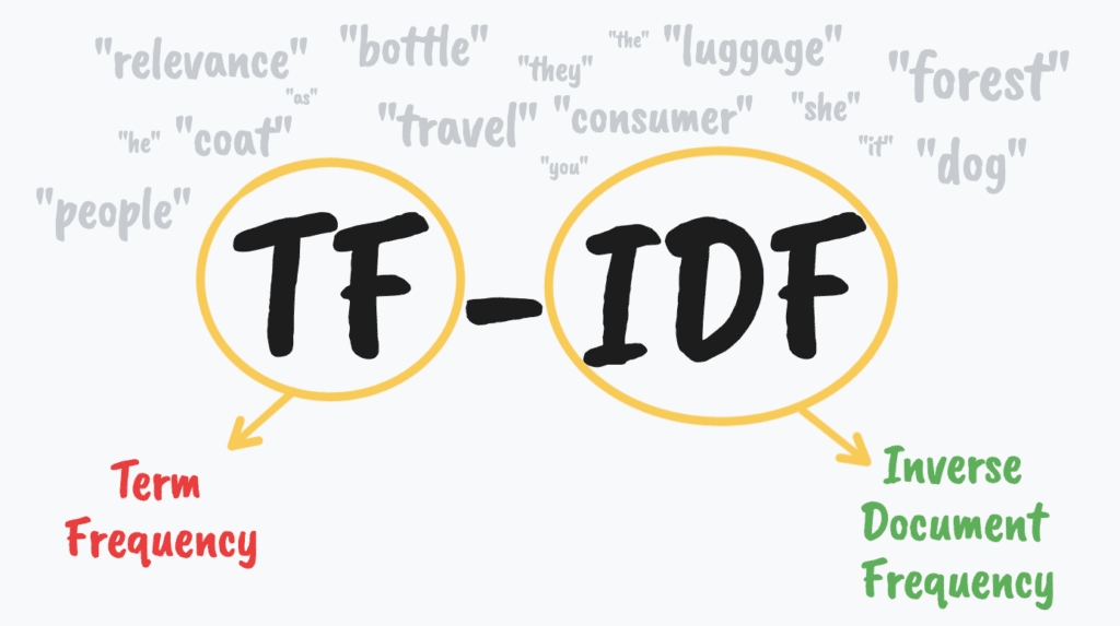
TF-IDF (Term Frequency-Inverse Document Frequency) is a numerical statistic used to reflect how important a word (term) is to a document in a collection or corpus. TF-IDF is a combination of two metrics: term frequency (TF) and inverse document frequency (IDF).

Term frequency measures how frequently a term \(t\) appears in a document \(d\) relative to the total number of terms in that document:

\[ \mathrm{TF}(t, d) = \frac{\text{Number of times term } t \text{ appears in document }d}{\text{Total number of terms in document }d}. \]

In other words,

\[ \mathrm{TF}(t, d) = \frac{n_{td}}{\sum\limits_{t' \in d} n_{t'd}} \]

where \(n_{td}\) is the number of times that term \(t\) occurs in document \(d\).

Note

Sometimes term frequencies are taken as raw counts \(n_{td}\): \(\mathrm{TF}(t, d) = n_{td}\).
IDF measures how important a term \(t\) is in the entire corpus \(D\):

\[ \mathrm{IDF}(t,D)= \log \frac{\text{Total number of documents in } D}{\text{Number of documents containing term } t}, \]

or

\[ \mathrm{IDF}(t,D)= \log \frac{\vert D \vert}{n_t}, \quad n_t = \vert \{d \in D \colon t \in d\}\vert. \]
Note

According to sklearn documentation, there are other forms for IDF:
- \(\mathrm{IDF}(t,D) = \log \frac{\vert D \vert}{n_t} + 1\)
- \(\mathrm{IDF}(t,D) = \log \frac{\vert D \vert}{n_t + 1}\)
- \(\mathrm{IDF}(t,D) = \log \frac{\vert D \vert + 1}{n_t + 1} + 1\)

Finally, TF-IDF of a term \(t\) and a documnent \(d\) from collection \(D\) is

(1)#\[ \text{TF-IDF}(t, d, D) = \mathrm{TF}(t, d) \times \mathrm{IDF}(t,D) = \frac{n_{td}}{\sum\limits_{t' \in d} n_{t'd}} \cdot \log \frac{\vert D \vert}{n_t}.\]

TF-IDF can serve as an alternative to the counts from BoW method. Let’s apply it to our toy example. First, build BoW count matrix automatically:

from sklearn.feature_extraction.text import CountVectorizer
import pandas as pd

sentences = [
    "I love machine learning",
    "Machine learning is fun",
    "I love programming",
    "Programming is fun",
    "Machine learning is important",
    "Math for fun",
    "Learning math is important for machine learning"
]

vectorizer = CountVectorizer(token_pattern=r"(?u)\b\w+\b")
BoW = vectorizer.fit_transform(sentences).todense() 
pd.DataFrame(data=BoW, columns=vectorizer.get_feature_names_out(), index=range(1, 8))

	for	fun	i	important	is	learning	love	machine	math	programming
1	0	0	1	0	0	1	1	1	0	0
2	0	1	0	0	1	1	0	1	0	0
3	0	0	1	0	0	0	1	0	0	1
4	0	1	0	0	1	0	0	0	0	1
5	0	0	0	1	1	1	0	1	0	0
6	1	1	0	0	0	0	0	0	1	0
7	1	0	0	1	1	2	0	1	1	0

Now calculate TF-IDF matrix:

from sklearn.feature_extraction.text import TfidfVectorizer
vectorizer = TfidfVectorizer(token_pattern=r"(?u)\b\w+\b", norm=None, smooth_idf=False)
tfidf = vectorizer.fit_transform(sentences).todense() 
pd.DataFrame(data=tfidf, columns=vectorizer.get_feature_names_out(), index=range(1, 8))

	for	fun	i	important	is	learning	love	machine	math	programming
1	0.000000	0.000000	2.252763	0.000000	0.000000	1.559616	2.252763	1.559616	0.000000	0.000000
2	0.000000	1.847298	0.000000	0.000000	1.559616	1.559616	0.000000	1.559616	0.000000	0.000000
3	0.000000	0.000000	2.252763	0.000000	0.000000	0.000000	2.252763	0.000000	0.000000	2.252763
4	0.000000	1.847298	0.000000	0.000000	1.559616	0.000000	0.000000	0.000000	0.000000	2.252763
5	0.000000	0.000000	0.000000	2.252763	1.559616	1.559616	0.000000	1.559616	0.000000	0.000000
6	2.252763	1.847298	0.000000	0.000000	0.000000	0.000000	0.000000	0.000000	2.252763	0.000000
7	2.252763	0.000000	0.000000	2.252763	1.559616	3.119232	0.000000	1.559616	2.252763	0.000000

Word embeddings#

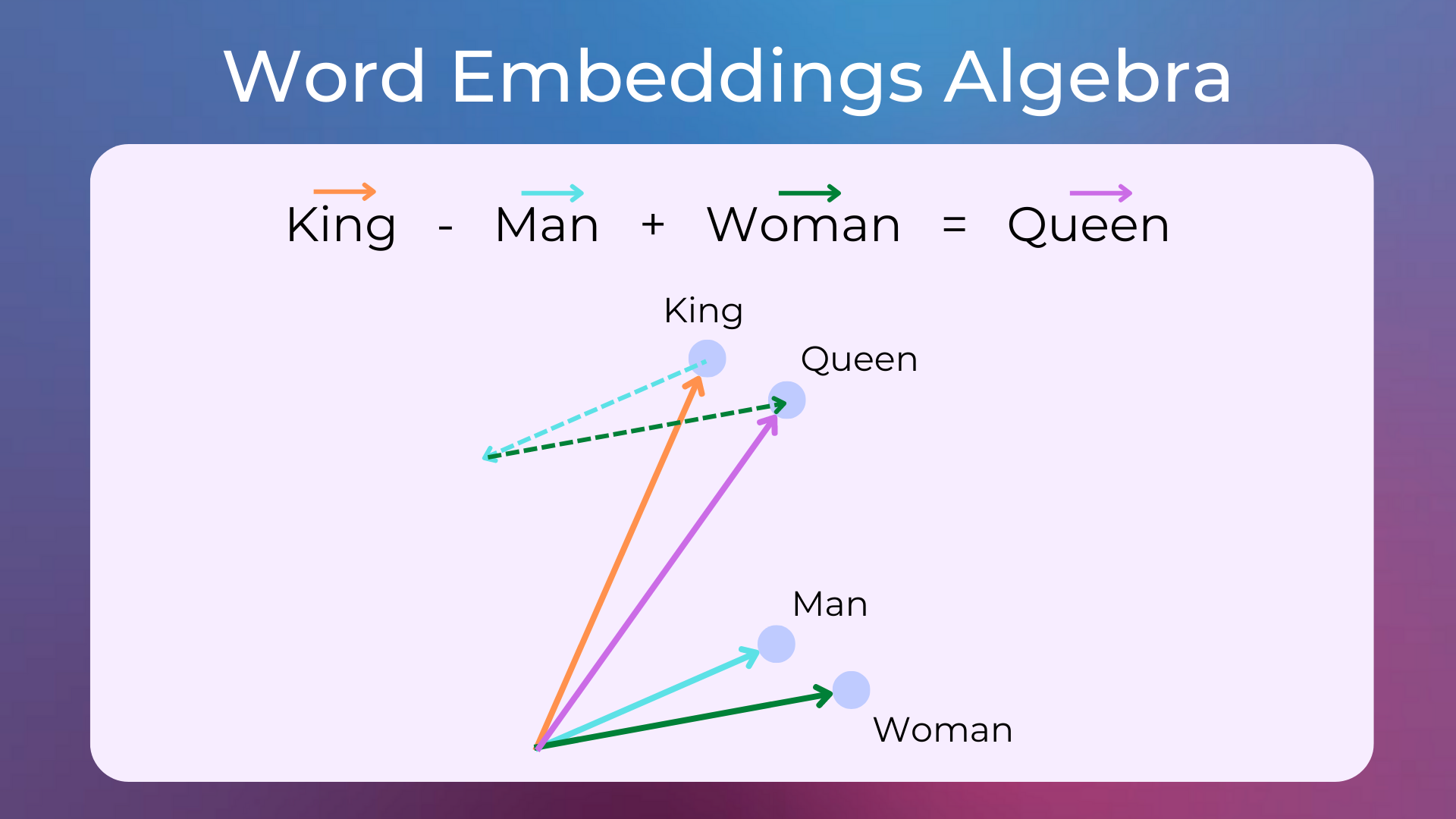
https://www.nlplanet.org/course-practical-nlp/_images/word2vec.png

Word embeddings are dense, low-dimensional vector representations of words that capture their meanings, relationships, and contexts in a continuous vector space. Unlike the sparse and high-dimensional vectors produced by BoW or TF-IDF models, word embeddings encode semantic information by placing semantically similar words closer together in the vector space.

Popular techniques for generating word embeddings:

word2vec
GloVe
fasttext
Transformer-based models (e.g., BERT)

Exercises#

Which disadvantages of BoW model could be overcomed by applying TF-IDF?
Can TF-IDF (1) be negative?
TF-IDF calculated by sklearn seems to be different from that of given by (1). Why?
Suppose that a term \(t\) is present in each document exactly once. What is the value of \(\text{TF-IDF}(t, d)\) for any document \(d\)? What if we use some modifications of (1)?

#Sentence	I	love	machine	learning	is	fun	programming	important	math	for
1	1	1	1	1	0	0	0	0	0	0
2	0	0	1	1	1	1	0	0	0	0
3	1	1	0	0	0	0	1	0	0	0
4	0	0	0	0	1	1	1	0	0	0
5	0	0	1	1	1	0	0	1	0	0
6	0	0	0	0	0	1	0	0	1	1
7	0	0	1	2	1	0	0	1	1	1

	for	fun	i	important	is	learning	love	machine	math	programming
1	0	0	1	0	0	1	1	1	0	0
2	0	1	0	0	1	1	0	1	0	0
3	0	0	1	0	0	0	1	0	0	1
4	0	1	0	0	1	0	0	0	0	1
5	0	0	0	1	1	1	0	1	0	0
6	1	1	0	0	0	0	0	0	1	0
7	1	0	0	1	1	2	0	1	1	0

#Sentence	I	love	machine	learning	is	fun	programming	important	math	for
1	1	1	1	1	0	0	0	0	0	0
2	0	0	1	1	1	1	0	0	0	0
3	1	1	0	0	0	0	1	0	0	0
4	0	0	0	0	1	1	1	0	0	0
5	0	0	1	1	1	0	0	1	0	0
6	0	0	0	0	0	1	0	0	1	1
7	0	0	1	2	1	0	0	1	1	1

	for	fun	i	important	is	learning	love	machine	math	programming
1	0	0	1	0	0	1	1	1	0	0
2	0	1	0	0	1	1	0	1	0	0
3	0	0	1	0	0	0	1	0	0	1
4	0	1	0	0	1	0	0	0	0	1
5	0	0	0	1	1	1	0	1	0	0
6	1	1	0	0	0	0	0	0	1	0
7	1	0	0	1	1	2	0	1	1	0