Training of MLP#
Learning objectives#
Binary classification#
The output of the neural network is usually a number from \([0, 1]\) which is the probability of the positive class. Sigmoid is the typical choice for the output layer:
Loss function:
Multiclass classification#
For \(K\) classes the output contains \(K\) numbers \((\widehat y_1, \ldots, \widehat y_K)\)
\(\widehat y_k\) is the probability of class \(k\)
Now the output of the neural network is
Finally, plug the predictions into the cross-entropy loss:
Regression#
Predict a real number \(\widehat y = x_L = x_{\mathrm{out}}\)
The loss function is usually quadratic:
Forward and backward pass#
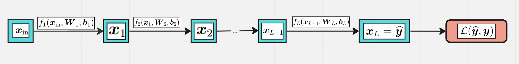
The goal is to minimize the loss function with respect to parameters \(\boldsymbol \theta\),
where
Let’s use the standard technique — the gradient descent!
Start from some random parameters \(\boldsymbol \theta_0\)
Given a training sample \((\boldsymbol x, \boldsymbol y)\), do the forward pass and get the output \(\boldsymbol {\widehat y} = F_{\boldsymbol \theta}(\boldsymbol x)\)
Calculate the loss function \(\mathcal L_{\boldsymbol\theta}(\boldsymbol {\widehat y}, \boldsymbol y)\)
Do the backward pass and calculate gradients
\[ \nabla_{\boldsymbol\theta}\mathcal L_{\boldsymbol\theta}(\boldsymbol {\widehat y}, \boldsymbol y) \]i.e.,
\[ \nabla_{\boldsymbol W_\ell}\mathcal L_{\boldsymbol\theta}(\boldsymbol {\widehat y}, \boldsymbol y) \text{ and } \nabla_{\boldsymbol b_\ell}\mathcal L_{\boldsymbol\theta}(\boldsymbol {\widehat y}, \boldsymbol y), \quad 1\leqslant \ell \leqslant L. \]Update the parameters:
Go to step 2 with next training sample
Batch training#
It is compuationally inefficient to update all the parameters every time after passing a training sample. Instead, take a batch of size \(B\) of training samples at a time and form the matrix \(\boldsymbol X_{\mathrm{in}}\) if the shape \(B\times n_0\). Now each hidden representation is a matrix of the shape \(B \times n_i\):
The output also has \(B\) rows. For instance, in the case of multiclassification task we have