Types of supervised learning

Given a labeled training dataset

(2)\[\mathcal D = \{(\boldsymbol x_i, y_i)\}_{i=1}^n, \quad \boldsymbol x_i \in \mathbb R^d, \quad y_i \in \mathcal Y,\]

we want to build a predictive model \(f_{\boldsymbol \theta}\colon \mathbb R^d\to \mathcal Y\) which is usually taken from some parametric family

\[ \mathcal F = \{f_{\boldsymbol \theta}(\boldsymbol x) \vert \boldsymbol \theta \in \mathbb R^m\}. \]

Dummy model

The simplest possible model is constant (dummy) model which always predicts the same value:

\[ \widehat y_i = f(\boldsymbol x_i) = c\in\mathcal Y \text{ for all } i = 1, \ldots, n.\]

A dummy model has no parameters (\(m=0\)) and does not require any training.

To fit a model means to find a value of \(\boldsymbol \theta\) which minimizes the loss function

\[ \mathcal L(\boldsymbol \theta) = \frac 1n \sum\limits_{i=1}^n \ell(f_{\boldsymbol \theta}(\boldsymbol x_i), y_i) \to \min \limits_{\boldsymbol \theta} \]

Depending on the set of targets \(\mathcal Y\) supervised learning is split into classification and regression.

Classification

If \(\mathcal Y\) is a finite set of categories, the predictive model \(f_{\boldsymbol \theta}\colon \mathbb R^d\to \mathcal Y\) is often called a classifier. In should classify inputs into several categories from \(\mathcal Y\).

Binary classification

In binary classification problems there are only two classes, which are often called positive and negative. The target set \(\mathcal Y\) in this case consists of two elements, and usually denoted as \(\mathcal Y = \{0, 1\}\) or \(\mathcal Y = \{-1, +1\}\).

Examples

• spam filtering (1 = spam, 0 = not spam)

• medical diagnosis (1 = sick, 0 = healthy)

• sentiment analysis (1 = positive, 0 = negative)

• credit card fraud detection (1 = fraudulent transaction, 0 = legitimate transaction)

• customer churn prediction (1 = cutomer leaves, 0 = customer stays)

Note

There’s no inherent rule that “positive” must correspond to a “good” outcome. Instead, it usually refers to the class of greater interest.

Loss function

Let \(\widehat y_i = f_{\boldsymbol \theta}(\boldsymbol x_i)\) be the prediction of the model on the \(i\)-th sample. A typical loss function for binary classification is misclassification rate (or error rate) — the fraction of incorrect predictions (misclassifications):

(3)\[ \mathcal L(\boldsymbol \theta) = \frac 1n \sum\limits_{i=1}^n \mathbb I\big[y_i \ne \hat y_i\big]\]

The error rate is not a smooth function, that’s why a binary classifier often predicts a number \(\tilde y \in (0, 1)\) which is treated as probability of positive class. In such case binary cross-entropy loss is used:

(4)\[ \mathcal L(\boldsymbol \theta) = -\frac 1n \sum\limits_{i=1}^n \big(y_i \log(\tilde y_i) + (1-y_i) \log(1 - \tilde y_i)\big)\]

Notation

1. By convention \(0\log 0 = 0\)

2. By default each \(\log\) has base \(e\)

3. Indicator \(\mathbb I[P]\) is defined as

\[\begin{split} \mathbb I[P] = \begin{cases} 1, & \text{ if } P \text{ is true} \\ 0, & \text{ if } P \text{ is false} \end{cases} \end{split}\]

Example

Suppose that true labels \(y\) and predictions \(\hat y\) are as follows:

Table 1 Binary classificaton

\(y\)	\(\hat y\)	\(\tilde y\)
\(0\)	\(0\)	\(0.2\)
\(0\)	\(1\)	\(0.6\)
\(1\)	\(0\)	\(0.3\)
\(1\)	\(1\)	\(0.9\)
\(0\)	\(0\)	\(0.1\)

Calculate the missclassification rate (3) and the binary cross-entropy loss (4).

Solution

There are \(2\) misclassifications, hence, the error rate equals \(\frac 25 = 0.4\). For the cross entropy loss we have

\[ \mathcal L = -\frac15\big(\log(1 - 0.2) + \log(1 - 0.6) + \log(0.3) + \log(0.9) + \log (1-0.1)\big) \approx 0.51. \]

W3sicXVlc3Rpb24iOiAiQ2FsY3VsYXRlIHRoZSBtaXNjbGFzc2lmaWNhdGlvbiByYXRlIiwgInR5cGUiOiAibnVtZXJpYyIsICJhbnN3ZXJzIjogW3sidHlwZSI6ICJ2YWx1ZSIsICJ2YWx1ZSI6IDAuNCwgImNvcnJlY3QiOiB0cnVlLCAiZmVlZGJhY2siOiAiUmlnaHQgeW91IGFyZSEgSGVyZSAkTj01JCwgdHdvIGluY29ycmVjdCBwcmVkaWN0aW9ucywgc28gdGhlIGxvc3MgaXMgJFxcZnJhYyAyNSQifSwgeyJ0eXBlIjogImRlZmF1bHQiLCAiZmVlZGJhY2siOiAiTm9wZSJ9XX0sIHsicXVlc3Rpb24iOiAiQ2FsY3VsYXRlIHRoZSBjcm9zcy1lbnRyb3B5IGxvc3MiLCAidHlwZSI6ICJtYW55X2Nob2ljZSIsICJhbnN3ZXJzIjogW3siYW5zd2VyIjogIiQwJCIsICJjb3JyZWN0IjogZmFsc2UsICJmZWVkYmFjayI6ICJUb28gbG93In0sIHsiYW5zd2VyIjogIiRcXGZyYWMgMTUgXFxsb2cgMiQiLCAiY29ycmVjdCI6IGZhbHNlLCAiZmVlZGJhY2siOiAiRG9lc24ndCBsb29rIGNvcnJlY3QifSwgeyJhbnN3ZXIiOiAiJFxcZnJhYyAxNSBcXGxvZyAzJCIsICJjb3JyZWN0IjogZmFsc2UsICJmZWVkYmFjayI6ICJOb3BlIn0sIHsiYW5zd2VyIjogIiQrXFxpbmZ0eSQiLCAiY29ycmVjdCI6IHRydWUsICJmZWVkYmFjayI6ICJPaCwgeWVhaC4uLiJ9XX1d

Multiclass classification

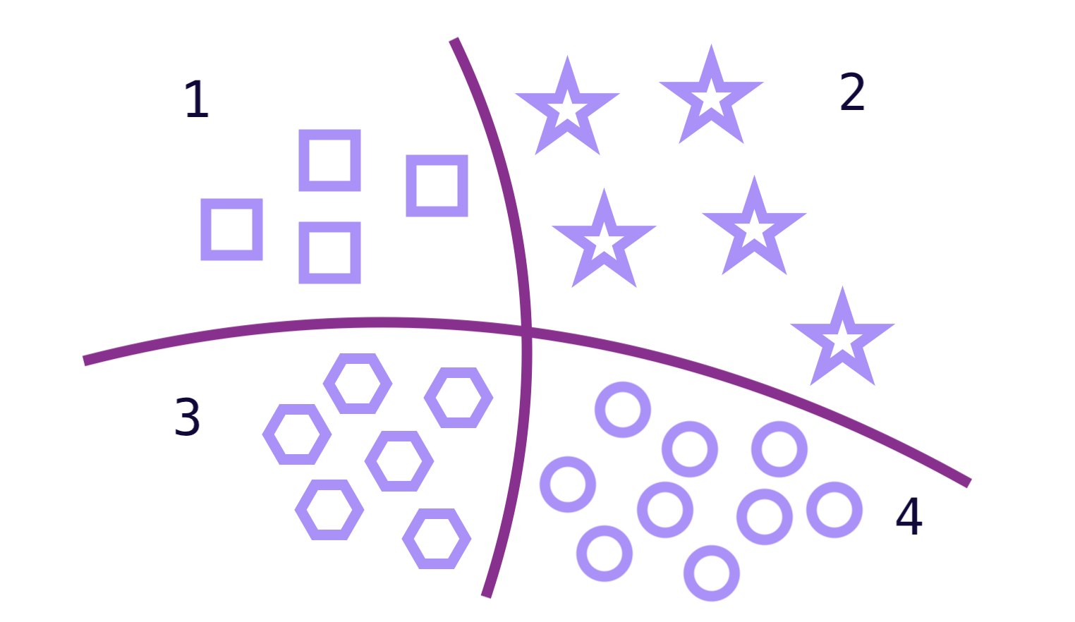
Quite often we need to categorize into several distance classes. Here are some examples:

• image classificaton (e.g., MNIST)

• language identification

• music genre detection

The error rate (3) is still valid if we have more than two classes \(\mathcal Y = \{1, 2, \ldots, K\}\). More often, a multiclass variant of (4) is used.

After applying one-hot encoding targets become \(K\)-dimensional vectors:

\[ \boldsymbol y_i \in \{0, 1\}^K,\quad \sum\limits_{k=1}^K y_{ik} = 1. \]

Now suppose that a classifier predicts a vector of probabilities of belonging to class \(k\):

\[ \hat{\boldsymbol y}_i = f_{\boldsymbol \theta}(\boldsymbol x_i) \in [0, 1]^K,\quad \hat y_{ik} = \mathbb P(\boldsymbol x_i \in \text{ class }k) \]

The cross-entropy loss is calculated as

(5)\[\mathcal L(\boldsymbol \theta) = -\frac 1n \sum\limits_{i=1}^n \sum\limits_{k=1}^Ky_{ik} \log(\hat y_{ik}).\]

Example

Classifying into \(3\) classes, model produces the following outputs:

\(y\)	\(\boldsymbol {\hat y}\)
\(0\)	\((0.25, 0.4, 0.35)\)
\(0\)	\((0.5, 0.3, 0.2)\)
\(1\)	\(\big(\frac 12 - \frac 1{2\sqrt 2}, \frac 1{\sqrt 2}, \frac 12 - \frac 1{2\sqrt 2}\big)\)
\(2\)	\((0, 0, 1)\)

Calculate the cross-entropy loss (5). Assume that log base is \(2\).

W3sicXVlc3Rpb24iOiAiQ2FsY3VsYXRlIHRoZSBjcm9zcyBlbnRyb3B5IGZyb20gdGhlIHByZXZpb3VzIGV4YW1wbGUiLCAidHlwZSI6ICJudW1lcmljIiwgImFuc3dlcnMiOiBbeyJ0eXBlIjogInZhbHVlIiwgInZhbHVlIjogMC44NzUsICJjb3JyZWN0IjogdHJ1ZSwgImZlZWRiYWNrIjogIkV4YWN0bHkhIn0sIHsidHlwZSI6ICJkZWZhdWx0IiwgImZlZWRiYWNrIjogIkluY29ycmVjdCJ9XX1d

Regression

If target set \(\mathcal Y\) is continuous (e.g., \(\mathcal Y = \mathbb R\) or \(\mathcal Y = \mathbb R^m\)) the predictive model \(f_{\boldsymbol \theta}\colon \mathbb R^d\to \mathcal Y\) is called a regression model or regressor.

The common choice for the loss on individual objects is quadratic loss

\[ \ell_2(\widehat y, y) = (y - \widehat y)^2 \]

The overall loss function is obtained by averaging over the training dataset (2):

\[ \mathcal L(\boldsymbol \theta) = \mathrm{MSE}(\boldsymbol \theta) = \frac 1n\sum\limits_{i=1}^n \ell_2(\widehat y_i, y_i) = \frac 1n\sum\limits_{i=1}^n (y_i - f_{\boldsymbol \theta}(\boldsymbol x_i))^2 \]

This loss is called mean squared error.

If the function \(f_{\boldsymbol \theta}(\boldsymbol x_i) = \boldsymbol {\theta^\mathsf{T} x}_i + b\) is linear, then the model is called linear regression. In case of one feature this is just a linear function of a single variable

\[ \widehat y_i = a x_i + b. \]

MSE loss equals to the average of sum of squares of the black line segments.

Exercises

1. Suppose we have a dataset (2) with categorical targets \(\mathcal Y = \{1 ,\ldots, K\}\). Let \(n_k\) be the size of the \(k\)-th category:

   \[ n_k = \sum\limits_{i=1}^n \mathbb I[y_i = k], \quad \sum\limits_{k=1}^K n_k = n. \]

   Consider a dummy model which always predicts category \(\ell\), \(1\leqslant \ell \leqslant K\). What is the value of the error rate (3)? For which \(\ell\) it is minimal?

2. Show that cross-entropy loss (5) turns into (4) if \(K=2\).

3. The MSE for a constant model \(f_{\boldsymbol \theta}(\boldsymbol x_i) = c\) is given by

   \[ \frac 1n \sum\limits_{i=1}^n (y_i - c)^2. \]

   For which \(c\) it is minimal?

4. How the answer to the previous problem will change if we replace MSE by MAE:

   \[ \frac 1n \sum\limits_{i=1}^n \vert y_i - c\vert \to \min \limits_c \]

5. How will the graph for linear regression look like in case of \(1\) or \(2\) points?