k-Nearest Neighbors

k-Nearest Neighbors is a nonparametric model. The idea is simple:

• choose hyperparameter \(k\in\mathbb N\);

• choose a distance metric in \(\mathbb R^d\) (for example, Euclidean);

• for a sample \(\boldsymbol x \in \mathbb R^d\) find its \(k\) nearest neighbors among the training dataset;

• classify or predict the label of \(\boldsymbol x\) according to the labels of its neighbors.

Distance between two vectors \(\boldsymbol x, \boldsymbol y \in \mathbb R^d\) is defined as norm of their difference

\[ \rho(\boldsymbol x, \boldsymbol y) = \Vert \boldsymbol x- \boldsymbol y\Vert. \]

See vector norm section for details.

k-NN algorithm

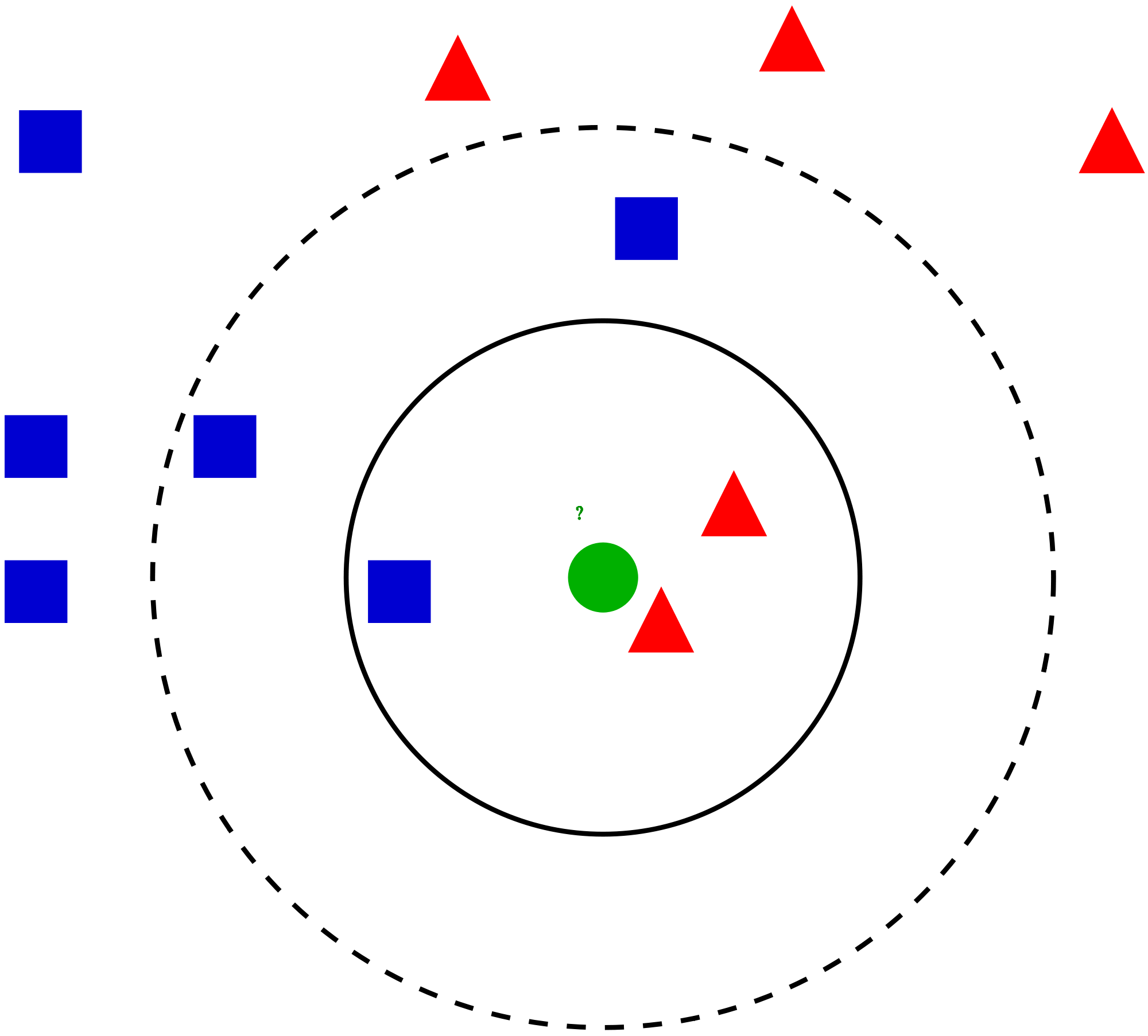
Fig. 1 Simple k-NN

Given the training dataset \(\{(\boldsymbol x_i, y_i)\}_{i=1}^n\), how to classify a new object \(\boldsymbol x\)?

1. Sort distances \(\rho (\boldsymbol x_i, \boldsymbol x)\) in increasing order:

   \[ \rho (\boldsymbol x_{(1)}, \boldsymbol x) \leqslant \rho (\boldsymbol x_{(2)}, \boldsymbol x) \leqslant \ldots \leqslant \rho (\boldsymbol x_{(n)}, \boldsymbol x) \]

2. So \(\boldsymbol x_{(i)}\) is the \(i\)-th neighbor of the object \(\boldsymbol x\)

3. Let \(y_{(i)}\) be the label of \(\boldsymbol x_{(i)}\)

4. The label \(\hat y\) of the object \(\boldsymbol x\in\mathbb R^d\) is set to the most common label among \(k\) neighbors of \(\boldsymbol x\):

\[ \widehat y = \arg\max_{y\in Y} \sum\limits_{i=1}^k \mathbb I[y = y_{(i)}] \]

For regression task the last step is subsituted by

\[ \widehat y = \frac 1k\sum\limits_{i=1}^k y_{(i)}. \]

Note that \(\widehat y = y_{(1)}\) if \(k=1\).

Voronoi tessellation

A k-NN classifier with \(k=1\) induces a Voronoi tessellation of the points. This is a partition of space which associates a region \(V(\boldsymbol x_i)\) with each sample \(\boldsymbol x_i\) in such a way that all points in \(V(\boldsymbol x_i)\) are closer to \(\boldsymbol x_i\) than to any other point. In other words,

\[ V(\boldsymbol x_i) = \{\boldsymbol z \in \mathbb R^n\colon \rho(\boldsymbol x_i, \boldsymbol z) < \rho(\boldsymbol x_j, \boldsymbol z) \text{ for all }j\ne i\}. \]

W3sicXVlc3Rpb24iOiAiU3VwcG9zZSB3ZSBhcmUgdHJhaW5pbmcgJDEkLU5OIGFsZ29yaXRobSB1c2luZyBtaXNjbGFzc2lmaWNhdGlvbiByYXRlIGFzIHRoZSBsb3NzIGZ1bmN0aW9uLiBXaGF0IHdpbGwgYmUgdGhlIHRyYWluIGVycm9yPyIsICJ0eXBlIjogIm51bWVyaWMiLCAiYW5zd2VycyI6IFt7InR5cGUiOiAidmFsdWUiLCAidmFsdWUiOiAwLCAiY29ycmVjdCI6IHRydWUsICJmZWVkYmFjayI6ICJSaWdodCBvbiEgQWxsIHRyYWluaW5nIHBvaW50cyB3aWxsIGJlIGNsYXNzaWZpZWQgY29ycmVjdGx5In0sIHsidHlwZSI6ICJyYW5nZSIsICJyYW5nZSI6IFstMTAwMDAwMDAwMDAwMDAwMDAwMDAwMDAwMDAwMDAwMDAwMDAwMDAwMDAwMDAwMDAwMDAwMDAwMDAwMDAwMDAwMDAwMDAwMDAwMDAwMDAwMDAwMDAwMDAwMDAwMDAwMDAwMDAwMDAwMDAwMDAwMDAwMDAwMDAwMDAwMDAwMDAwMDAwMDAwMDAwMDAwMDAwMDAwMDAwMDAwMDAwMDAwMDAwMDAwMDAwMDAwMDAwMDAwMDAwMDAwMDAwMDAwMDAwMDAwMDAwMDAwMDAwMDAwMDAwMDAwMDAwMDAwMDAwMDAwMDAwMDAwMDAwMDAwMDAwMDAwMDAwMDAwMDAwMDAwMDAwMDAwMDAwMDAwMDAwMDAwMDAwMDAwMDAwMDAwMDAwMDAwMDAwMDAwMDAwMDAwMCwgMF0sICJmZWVkYmFjayI6ICJNaXNjbGFzc2lmaWNhdGlvbiByYXRlIG11c3QgYmUgYmV0d2VlbiAwIGFuZCAxIn0sIHsidHlwZSI6ICJyYW5nZSIsICJyYW5nZSI6IFsxLjAwMDAwMDAwMDEsIDEwMDAwMDAwMDAwMDAwMDAwMDAwMDAwMDAwMDAwMDAwMDAwMDAwMDAwMDAwMDAwMDAwMDAwMDAwMDAwMDAwMDAwMDAwMDAwMDAwMDAwMDAwMDAwMDAwMDAwMDAwMDAwMDAwMDAwMDAwMDAwMDAwMDAwMDAwMDAwMDAwMDAwMDAwMDAwMDAwMDAwMDAwMDAwMDAwMDAwMDAwMDAwMDAwMDAwMDAwMDAwMDAwMDAwMDAwMDAwMDAwMDAwMDAwMDAwMDAwMDAwMDAwMDAwMDAwMDAwMDAwMDAwMDAwMDAwMDAwMDAwMDAwMDAwMDAwMDAwMDAwMDAwMDAwMDAwMDAwMDAwMDAwMDAwMDAwMDAwMDAwMDAwMDAwMDAwMDAwMDAwMDAwMDAwMDAwMDAwMDBdLCAiZmVlZGJhY2siOiAiTWlzY2xhc3NpZmljYXRpb24gcmF0ZSBtdXN0IGJlIGJldHdlZW4gMCBhbmQgMSJ9LCB7InR5cGUiOiAiZGVmYXVsdCIsICJmZWVkYmFjayI6ICJObywgdGhpcyBpcyBub3QgdHJ1ZSJ9XX1d

Role of \(k\)

The decision boundaries become smoother as \(k\) grows. Here is an example from [Murphy, 2022] (figure 16.2): k-NN algorithm is applied to simulated data with three clusters.

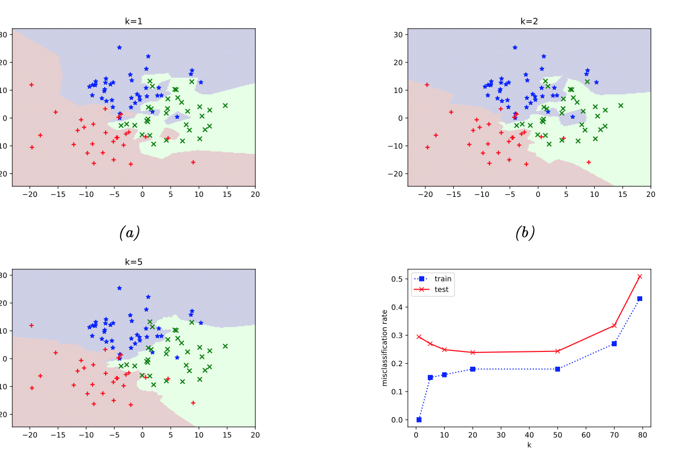
Q. Look at the graph of train and test errors. For which values of \(k\) we can suspect overfitting?

Effective number of parameters of \(k\)-NN

It is equal to \(\frac n k\). To get an idea of why, note that if the neighborhoods were nonoverlapping, there would be \(\frac nk\) neighborhoods and we would fit one parameter (a mean) in each neighborhood ([Hastie et al., 2009], p. 14)

Curse of dimensionality

Only red part of watermelon is useful, and watermelon rind is thrown away. Suppose that the watermelon is a ball of radius \(R\), and the length of the rind is \(10\%\) of \(R\).

W3sicXVlc3Rpb24iOiAiV2hhdCBwZXJjZW50YWdlIG9mIHRoZSB3YXRlcm1lbG9uIGlzIGVhdGFibGU/IiwgInR5cGUiOiAibnVtZXJpYyIsICJhbnN3ZXJzIjogW3sidHlwZSI6ICJ2YWx1ZSIsICJ2YWx1ZSI6IDAuNzI5LCAiY29ycmVjdCI6IGZhbHNlLCAiZmVlZGJhY2siOiAiVGhpcyBpcyB0aGUgcGFydCB3cml0dGVuIGFzIGRlY2ltYWwgZnJhY3Rpb24ifSwgeyJ0eXBlIjogInZhbHVlIiwgInZhbHVlIjogNzIuOSwgImNvcnJlY3QiOiB0cnVlLCAiZmVlZGJhY2siOiAiVGhhdCdzIGNvcnJlY3QhICQoMC45KV4zXFx0aW1lcyAxMDBcXCUgPSA3Mi45XFwlJCJ9LCB7InR5cGUiOiAicmFuZ2UiLCAicmFuZ2UiOiBbLTEwMDAwMDAwMDAwMDAwMDAwMDAwMDAwMDAwMDAwMDAwMDAwMDAwMDAwMDAwMDAwMDAwMDAwMDAwMDAwMDAwMDAwMDAwMDAwMDAwMDAwMDAwMDAwMDAwMDAwMDAwMDAwMDAwMDAwLCAwXSwgImZlZWRiYWNrIjogIlBlcmNlbnRhZ2UgY2Fubm90IGJlIG5lZ2F0aXZlIn0sIHsidHlwZSI6ICJyYW5nZSIsICJyYW5nZSI6IFsxMDAuMDAwMDAwMDAwMSwgMTAwMDAwMDAwMDAwMDAwMDAwMDAwMDAwMDAwMDAwMDAwMDAwMDAwMDAwMDAwMDAwMDAwMDAwMDAwMDAwMDAwMDAwMDAwMDAwMDAwMDAwMDAwMDAwMDAwMDAwMDAwMDAwMDAwMDBdLCAiZmVlZGJhY2siOiAiWW91IGNhbm5vdCBlYXQgbW9yZSB0aGF0ICQxMDBcXCUkIG9mIHRoZSB3YXRlcm1lbG9uIn0sIHsidHlwZSI6ICJkZWZhdWx0IiwgImZlZWRiYWNrIjogIk5vLCB0aGlzIGlzIG5vdCB0cnVlIn1dfSwgeyJxdWVzdGlvbiI6ICJIb3cgdGhlIGFuc3dlciB3b3VsZCBjaGFuZ2UgaWYgd2Ugd2VyZSBsaXZpbmcgaW4gJFxcbWF0aGJiIFJeezEwfSQ/IiwgInR5cGUiOiAibnVtZXJpYyIsICJhbnN3ZXJzIjogW3sidHlwZSI6ICJyYW5nZSIsICJyYW5nZSI6IFswLjM0OCwgMC4zNDkxXSwgImNvcnJlY3QiOiBmYWxzZSwgImZlZWRiYWNrIjogIlRoaXMgaXMgdGhlIHBhcnQgd3JpdHRlbiBhcyBkZWNpbWFsIGZyYWN0aW9uIn0sIHsidHlwZSI6ICJyYW5nZSIsICJyYW5nZSI6IFszNC44LCAzNC45MV0sICJjb3JyZWN0IjogdHJ1ZSwgImZlZWRiYWNrIjogIlRoYXQncyBjb3JyZWN0ISAkKDAuOSleezEwfVxcdGltZXMgMTAwXFwlIFxcYXBwcm94IDM0LjlcXCUkIn0sIHsidHlwZSI6ICJyYW5nZSIsICJyYW5nZSI6IFstMTAwMDAwMDAwMDAwMDAwMDAwMDAwMDAwMDAwMDAwMDAwMDAwMDAwMDAwMDAwMDAwMDAwMDAwMDAwMDAwMDAwMDAwMDAwMDAwMDAwMDAwMDAwMDAwMDAwMDAwMDAwMDAwMDAwMDAsIDBdLCAiY29ycmVjdCI6IGZhbHNlLCAiZmVlZGJhY2siOiAiUGVyY2VudGFnZSBjYW5ub3QgYmUgbmVnYXRpdmUifSwgeyJ0eXBlIjogInJhbmdlIiwgInJhbmdlIjogWzEwMC4wMDAwMDAwMDAxLCAxMDAwMDAwMDAwMDAwMDAwMDAwMDAwMDAwMDAwMDAwMDAwMDAwMDAwMDAwMDAwMDAwMDAwMDAwMDAwMDAwMDAwMDAwMDAwMDAwMDAwMDAwMDAwMDAwMDAwMDAwMDAwMDAwMDAwMF0sICJjb3JyZWN0IjogZmFsc2UsICJmZWVkYmFjayI6ICJZb3UgY2Fubm90IGVhdCBtb3JlIHRoYXQgJDEwMFxcJSQgb2YgdGhlIHdhdGVybWVsb24ifSwgeyJ0eXBlIjogImRlZmF1bHQiLCAiZmVlZGJhY2siOiAiRmFsc2UifV19XQ==

This is how the curse of dimensionality works. In \(50\)-dimensional space there is almost nothing to eat in a watermelon.

What are the consequenes of curse of the dimensionality for \(k\)-NN?

A common example from textbooks

Suppose we apply a \(k\)-NN classifier to data where the inputs are uniformly distributed in the \(d\)-dimensional unit cube. Suppose we estimate the density of class labels around a test point \(\boldsymbol x\) by “growing” a hyper-cube around \(\boldsymbol x\) until it contains a desired fraction \(p\) of the data points. The expected edge length of this cube will be \(e_d(p)=p^{\frac 1d}\) (see [Murphy, 2022], p. 530-531). For example, if \(d=10\) and we want to capture \(1\%\) of neighbours, we need extend the cube \(e_{10}(0.01) \approx 0.63\) along each dimension around \(\boldsymbol x\).

k-NN for Boston dataset

Load Boston dataset:

import pandas as pd

boston_df = pd.read_csv("../datasets/ISLP/Boston.csv").drop("Unnamed: 0", axis=1)
boston_df.head()

	crim	zn	indus	chas	nox	rm	age	dis	rad	tax	ptratio	lstat	medv
0	0.00632	18.0	2.31	0	0.538	6.575	65.2	4.0900	1	296	15.3	4.98	24.0
1	0.02731	0.0	7.07	0	0.469	6.421	78.9	4.9671	2	242	17.8	9.14	21.6
2	0.02729	0.0	7.07	0	0.469	7.185	61.1	4.9671	2	242	17.8	4.03	34.7
3	0.03237	0.0	2.18	0	0.458	6.998	45.8	6.0622	3	222	18.7	2.94	33.4
4	0.06905	0.0	2.18	0	0.458	7.147	54.2	6.0622	3	222	18.7	5.33	36.2

Split it into feature matrix \(\boldsymbol X\) and labels \(\boldsymbol y\):

X = boston_df.drop("medv", axis=1)
y = boston_df["medv"]
boston_df.shape, X.shape, y.shape

((506, 13), (506, 12), (506,))

Import kNN model from sklearn, and do fit-predict:

from sklearn.neighbors import KNeighborsRegressor

model = KNeighborsRegressor(n_neighbors=3)
model.fit(X, y)
y_hat = model.predict(X)
y_hat.shape

(506,)

Check MSE:

from sklearn.metrics import mean_squared_error

print("MSE loss:", mean_squared_error(y, y_hat))

MSE loss: 15.09318620992534

Study how MSE depends on the value of \(k\) — number of neighbors:

for n_neighbors in range(1, 11):
    model = KNeighborsRegressor(n_neighbors=n_neighbors)
    model.fit(X, y)
    y_hat = model.predict(X)
    print(f"MSE loss for {n_neighbors}-NN:", mean_squared_error(y, y_hat))

MSE loss for 1-NN: 0.0
MSE loss for 2-NN: 9.920642292490117
MSE loss for 3-NN: 15.09318620992534
MSE loss for 4-NN: 18.02147233201581
MSE loss for 5-NN: 20.895541501976286
MSE loss for 6-NN: 22.503348155467723
MSE loss for 7-NN: 23.99821368072921
MSE loss for 8-NN: 24.42564785079051
MSE loss for 9-NN: 25.821026204069682
MSE loss for 10-NN: 27.524774703557313

Looks like \(1\)-NN model is the best. Is it true?

To evaluate a model, one needs to split the dataset into train and test:

from sklearn.model_selection import train_test_split

X_train, X_test, y_train, y_test = train_test_split(X, y)
X_train.shape, y_train.shape, X_test.shape, y_test.shape

((379, 12), (379,), (127, 12), (127,))

Search for optimal number of neighbors:

train_loss = []
test_loss = []
ks = np.arange(1, 21)
for n_neighbors in ks:
    model = KNeighborsRegressor(n_neighbors=n_neighbors)
    model.fit(X_train, y_train)
    train_loss.append(mean_squared_error(y_train, model.predict(X_train)))
    test_loss.append(mean_squared_error(y_test, model.predict(X_test)))

plt.plot(ks, train_loss, lw=2, c='r', label="Train")
plt.plot(ks, test_loss, lw=2, c='b', label="Test")
plt.xlim(ks[0], ks[-1])
plt.xticks(ks)
plt.title("Train and test error for k-NN model")
plt.xlabel("k")
plt.ylabel("MSE")
plt.legend()
plt.grid(ls=":");

k-NN for classification

Load a simple digit dataset:

from sklearn.datasets import load_digits

digits = load_digits()
digits.data.shape, digits.target.shape

((1797, 64), (1797,))

Count samples of each class:

np.unique(digits.target, return_counts=True)

(array([0, 1, 2, 3, 4, 5, 6, 7, 8, 9]),
 array([178, 182, 177, 183, 181, 182, 181, 179, 174, 180]))

X_train, X_test, y_train, y_test = train_test_split(digits.data, digits.target)

Train a k-NN classifier for different values of \(k\):

from sklearn.neighbors import KNeighborsClassifier
from sklearn.metrics import accuracy_score

train_acc = []
test_acc = []
ks = np.arange(1, 31)
for n_neighbors in ks:
    model = KNeighborsClassifier(n_neighbors=n_neighbors)
    model.fit(X_train, y_train)
    train_acc.append(accuracy_score(y_train, model.predict(X_train)))
    test_acc.append(accuracy_score(y_test, model.predict(X_test)))

plt.plot(ks, train_acc, lw=2, c='r', label="Train")
plt.plot(ks, test_acc, lw=2, c='b', label="Test")
plt.xlim(ks[0], ks[-1])
plt.xticks(ks[::2])
plt.title("Train and test accuracy for k-NN model")
plt.xlabel("k")
plt.ylabel("accuracy")
plt.legend()
plt.grid(ls=":");

Exercises

1. What is the predicted label of the green cirle in Fig. 1 by the k-NN model if \(k=1\)? \(k=3\)? \(k=5\)? \(k=11\)?

2. Show that \(\Vert \boldsymbol x \Vert_\infty = \max\{\vert x_1\vert, \ldots, \vert x_d\vert\}\), i.e.,

   \[ \lim\limits_{p\to +\infty} \Big(\sum\limits_{i=1}^d |x_i|^p \Big)^{\frac 1p} = \max\{\vert x_1\vert, \ldots, \vert x_d\vert\}. \]

3. Consider a model binary classification problem with one feature and two objects of the training set: \(x_{1} = 0.2\), \(x_2 = 0.7\). The first object belongs to the first class, the second — to the second. Let’s add a new noise feature to the objects, uniformly distributed on the segment \([0, 1]\). Now each object is described by two float numbers. Let it be required to classify a new object \(u = (0, 0)\) in this space by the one nearest neighbor method with the Euclidean metric. What is the probability that, after adding noise, the second object will be closer to the object \(u\) than the first one?