Back propagation

Outline:

• Make the forward pass and calculate all hidden representations along with output and loss function:

\[ \boldsymbol X_1, \boldsymbol X_2, \ldots \boldsymbol X_{L-1}, \boldsymbol X_L = \boldsymbol{\widehat Y}, \mathcal L(\boldsymbol {\widehat Y}, \boldsymbol Y) \]

• Calculate the gradient of the loss function with respect to the output:

\[ \nabla_{\boldsymbol X_L} \mathcal L(\boldsymbol X_L, \boldsymbol Y) \]

• Make the backward pass from \(\boldsymbol X_{L-1}\) to \(\boldsymbol X_1\) and calculate \(\nabla_{\boldsymbol X_i}\mathcal L\), \(\nabla_{\boldsymbol W_i} \mathcal L\), \(\nabla_{\boldsymbol B_i}\mathcal L\) on each step

Backprop through one layer

All you need is… chain rule!

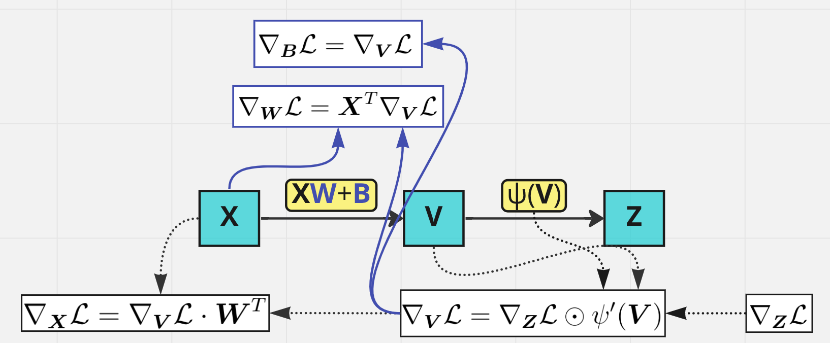
Backprop through activation layer

Suppose that we know the upstream gradient \(\nabla_{\boldsymbol Z}\mathcal L(\boldsymbol Z)\). The goal is to derive the formula for the downstream gradient \(\nabla_{\boldsymbol V}\tilde{\mathcal L}(\boldsymbol V)\) where \(\tilde{\mathcal L}(\boldsymbol V)=\mathcal L(\psi(\boldsymbol V))\). According to matrix calculus rules

\[ d\tilde{\mathcal L}(\boldsymbol V) = \mathrm{tr}\big(\nabla \tilde{\mathcal L}(\boldsymbol V)^\mathsf{T} d\boldsymbol V\big) = \mathrm{tr}\big(\nabla \mathcal L(\boldsymbol Z)^\mathsf{T} d\boldsymbol Z\big). \]

From (65) we know that \(d \boldsymbol Z = d\psi(\boldsymbol V) = \psi'(\boldsymbol V) \odot d\boldsymbol V = d\boldsymbol V \odot \psi'(\boldsymbol V)\). Hence,

\[ \mathrm{tr}\big(\nabla \mathcal L(\boldsymbol Z)^\mathsf{T} d\boldsymbol Z\big) = \mathrm{tr}\big(\nabla \mathcal L(\boldsymbol Z)^\mathsf{T} (\psi'(\boldsymbol V) \odot d\boldsymbol V)\big) \]

Exercise

Let \(\boldsymbol A, \boldsymbol B, \boldsymbol C \in \mathbb R^{m\times n}\). Show that

\[ \mathrm{tr}\big(\boldsymbol A^\mathsf{T} (\boldsymbol B \odot \boldsymbol C)\big) = \mathrm{tr}\big((\boldsymbol A \odot \boldsymbol B)^\mathsf{T} \boldsymbol C\big) \]

From this exercise we obtain

\[ d\tilde{\mathcal L}(\boldsymbol V) = \mathrm{tr}\big(\big(\nabla \mathcal L(\boldsymbol Z) \odot \psi'(\boldsymbol V)\big)^\mathsf{T} d\boldsymbol V\big), \]

and \(\nabla_{\boldsymbol V}\tilde{\mathcal L}(\boldsymbol V) = \nabla \mathcal L(\boldsymbol Z) \odot \psi'(\boldsymbol V)\).

Backprop through linear layer

Now our upstream gradient is \(\nabla_{\boldsymbol V}\mathcal L(\boldsymbol V)\), and we want to find the downstream gradient \(\nabla_{\boldsymbol X}\tilde{\mathcal L}(\boldsymbol X, \boldsymbol W, \boldsymbol B)\) where \(\tilde{\mathcal L}(\boldsymbol X, \boldsymbol W, \boldsymbol B)=\mathcal L(\boldsymbol{XW} + \boldsymbol B)\). Moreover, we also need formulas for \(\nabla_{\boldsymbol W}\tilde{\mathcal L}(\boldsymbol X, \boldsymbol W, \boldsymbol B)\) and \(\nabla_{\boldsymbol B}\tilde{\mathcal L}(\boldsymbol X, \boldsymbol W, \boldsymbol B)\) in order to make the gradient step.

Once again use chain rule and simple facts from calculus:

\[ d\tilde{\mathcal L}(\boldsymbol X) = \mathrm{tr}\big(\nabla \mathcal L(\boldsymbol V)^\mathsf{T} d\boldsymbol V\big) = \mathrm{tr}\big(\nabla \mathcal L(\boldsymbol V)^\mathsf{T} d\boldsymbol X \cdot \boldsymbol W\big) = \mathrm{tr}\big(\boldsymbol W\cdot\nabla \mathcal L(\boldsymbol V)^\mathsf{T} d\boldsymbol X \big), \]

\[ d\tilde{\mathcal L}(\boldsymbol W) = \mathrm{tr}\big(\nabla \mathcal L(\boldsymbol V)^\mathsf{T} d\boldsymbol V\big) = \mathrm{tr}\big(\nabla \mathcal L(\boldsymbol V)^\mathsf{T} \boldsymbol X d\boldsymbol W\big), \]

\[ d\tilde{\mathcal L}(\boldsymbol B) = \mathrm{tr}\big(\nabla \mathcal L(\boldsymbol V)^\mathsf{T} d\boldsymbol V\big) = \mathrm{tr}\big(\nabla \mathcal L(\boldsymbol V)^\mathsf{T} d\boldsymbol B\big) \]

Hence,

\[ \nabla_{\boldsymbol X}\tilde{\mathcal L} = \nabla\mathcal L(\boldsymbol V) \boldsymbol W^\mathsf{T}, \quad \nabla_{\boldsymbol W}\tilde{\mathcal L} = \boldsymbol X^\mathsf{T} \nabla\mathcal L(\boldsymbol V), \quad \nabla_{\boldsymbol B}\tilde{\mathcal L} = \nabla \mathcal L(\boldsymbol V). \]

Problem with bias

Usually bias is a vector, not matrix. If \(\boldsymbol X \in \mathbb R^{B\times m}\), \(\boldsymbol W \in \mathbb R^{m\times n}\) then bias is \(\boldsymbol b \in \mathbb R^{n}\), and linear layer looks like

\[\begin{split} \boldsymbol{XW} + \boldsymbol B, \quad \boldsymbol B = \begin{pmatrix} \boldsymbol b^\mathsf{T} \\ \vdots \\ \boldsymbol b^\mathsf{T} \end{pmatrix} \end{split}\]

Therefore, we want to find \(\nabla_{\boldsymbol b}\tilde{\mathcal L}\), which is also not matrix, but vector. It can be found from the equality

\[ d\tilde{\mathcal L}(\boldsymbol b) = \nabla_{\boldsymbol b} \tilde{\mathcal L}^\mathsf{T} d\boldsymbol b. \]

Denote

\[\begin{split} \nabla \mathcal L(\boldsymbol V) = \boldsymbol A = \begin{pmatrix} \boldsymbol a_1^\mathsf{T} \\ \vdots \\ \boldsymbol a_B^\mathsf{T} \end{pmatrix} \in \mathbb R^{B\times n}, \end{split}\]

then

\[\begin{split} d\tilde{\mathcal L}(\boldsymbol b) = \mathrm{tr}\big(\boldsymbol A^\mathsf{T} d\boldsymbol B\big) = = \mathrm{tr}\left([\boldsymbol a_1 \ldots \boldsymbol a_B] \begin{pmatrix}d\boldsymbol b^\mathsf{T} \\ \vdots \\ d\boldsymbol b^\mathsf{T} \end{pmatrix}\right) = \sum\limits_{i=1}^B \mathrm{tr}(\boldsymbol a_i d\boldsymbol b^\mathsf{T}) \end{split}\]

Since \(\mathrm{tr}(\boldsymbol a_i d\boldsymbol b^\mathsf{T}) = \mathrm{tr}(d\boldsymbol b^\mathsf{T}\boldsymbol a_i) = d\boldsymbol b^\mathsf{T}\boldsymbol a_i = \boldsymbol a_i^\mathsf{T}d\boldsymbol b\), we finally get

\[ d\tilde{\mathcal L}(\boldsymbol b) = \sum\limits_{i=1}^B \boldsymbol a_i^\mathsf{T}d\boldsymbol b = \Big(\underbrace{\sum\limits_{i=1}^B \boldsymbol a_i}_{\nabla\tilde{\mathcal L}(\boldsymbol b)}\Big)^\mathsf{T} d\boldsymbol b. \]

Hence, the downstream gradient \(\nabla\tilde{\mathcal L}(\boldsymbol b)\) is equal to the sum of the rows of the upstream gradient \(\nabla \mathcal L(\boldsymbol V)\).

Backprop through loss function

Regression

The most common choice for (multiple) regression is MSE: if target is \(\boldsymbol Y \in \mathbb R^{B\times m}\), model output is \(\widehat{\boldsymbol Y} \in \mathbb R^{B\times m}\), then

\[ \mathcal L(\boldsymbol Y, \widehat{\boldsymbol Y}) = \frac 1{Bm} \Vert \boldsymbol Y - \widehat{\boldsymbol Y}\Vert_F^2 = \frac 1{Bm}\sum\limits_{i=1}^B\sum\limits_{j=1}^m (Y_{ij} - \widehat Y_{ij})^2. \]

Since \(\Vert \boldsymbol Y - \widehat{\boldsymbol Y}\Vert_F^2 = \mathrm{tr}\big((\boldsymbol Y - \widehat{\boldsymbol Y})^\mathsf{T}(\boldsymbol Y - \widehat{\boldsymbol Y})\big)\),

\[ d\mathcal L(\boldsymbol Y, \widehat{\boldsymbol Y}) = \frac2{Bm} \mathrm{tr}\big((\widehat{\boldsymbol Y}-\boldsymbol Y )^\mathsf{T}\widehat{\boldsymbol Y}\big). \]

Consequently,

\[ \nabla_{\widehat{\boldsymbol Y}} \mathcal L(\boldsymbol Y, \widehat{\boldsymbol Y}) = \frac2{Bm} (\widehat{\boldsymbol Y}-\boldsymbol Y). \]

Sometimes they use sum of squares instead of MSE, then the multiplier \(\frac 1{Bm}\) is omitted.

Classification

The usual choice of loss here is cross-entropy loss:

(35)\[ \mathcal L(\boldsymbol Y, \boldsymbol {\widehat Y}) = -\frac 1N \sum\limits_{i=1}^N\sum\limits_{j=1}^K Y_{ij} \log \widehat Y_{ij} = -\frac 1N \mathrm{tr}\big(\boldsymbol Y^T\log\boldsymbol {\widehat Y}\big).\]

The target matrix \(\boldsymbol Y \in \mathbb R^{B\times K}\) consists of one-hot encoded rows, each of which contains \(1\) one and \(K-1\) zeros. Each row of the prediction matrix \(\boldsymbol {\widehat Y} \in \mathbb R^{B\times K}\) must be a valid probability distribution, which is achived by applying Softmax:

(36)\[ \widehat Y_{ij} = \mathrm{Softmax}(\boldsymbol X^{\mathrm{out}})_{ij} = \frac{e^{X^{\mathrm{out}}_{ij}}}{\sum\limits_{k=1}^K e^{X^{\mathrm{out}}_{ik}}}.\]

Формально Softmax и кросс-энтропия — это два подряд идущих слоя, однако, на практике в целях повышения вычислительной стабильности их часто объединяют в один (например, в pytorch Softmax и поэлементное взятие логарифма объединены в один слой LogSoftmax).

Plugging (36) into (35), we obtain

\[ \mathcal L\big(\boldsymbol Y, \mathrm{Softmax}(\boldsymbol X^{\mathrm{out}})\big) = -\frac 1N \sum\limits_{i=1}^N\sum\limits_{j=1}^K Y_{ij} \Big(X^{\mathrm{out}}_{ij} - \log\Big(\sum\limits_{k=1}^K e^{X^{\mathrm{out}}_{ik}}\Big)\Big). \]

Now differentiate it with respect to \(X_{mn}\):

\[ \frac{\partial \mathcal L}{\partial X_{mn}^{\mathrm{out}}} = -\frac 1N \sum\limits_{i=1}^N\sum\limits_{j=1}^K Y_{ij} \bigg(\delta_{im}\delta_{jn} - \frac{e^{X^{\mathrm{out}}_{in}}\delta_{im}}{\sum_{k=1}^K e^{X^{\mathrm{out}}_{ik}}}\bigg), \]

where \(\delta_{ij}\) is Kronecker delta. Since target matrix \(\boldsymbol Y\) enjoys the property \(\sum\limits_{j=1}^K Y_{ij} = 1\) for all \(i=1,\ldots, B\), we get

\[ \frac{\partial \mathcal L}{\partial X_{mn}^{\mathrm{out}}} = -\frac 1N Y_{mn} + \frac 1N \sum\limits_{j=1}^K Y_{mj} \frac{e^{X_{mn}^{\mathrm{out}}}}{\sum\limits_{k=1}^K e^{X^{\mathrm{out}}_{mk}}} = \frac 1N\big(\mathrm{Softmax}(\boldsymbol X^{\mathrm{out}})_{mn} - Y_{mn}\big). \]

Hence,

\[ \nabla_{\boldsymbol X^{\mathrm{out}}}\mathcal L(\boldsymbol Y, \widehat{\boldsymbol Y}) = \frac 1N\big(\widehat{\boldsymbol Y} - \boldsymbol Y\big)= \frac 1N\big(\mathrm{Softmax}(\boldsymbol X^{\mathrm{out}}) - \boldsymbol Y\big). \]