Estimations

Bias

Let \(X_1, \ldots, X_n\) be an i.i.d. sample from some distribution \(F_\theta(x)\). Estimation \(\widehat\theta = \widehat\theta (X_1, \ldots, X_n)\) of \(\theta\) is called unbiased if \(\mathbb E \widehat\theta = \theta\). Otherwise \(\widehat\theta\) is called biased, and its bias equals to

\[ \mathrm{bias}(\widehat \theta) = \mathbb E \widehat\theta - \theta. \]

For example, sample average \(\widehat\theta = \overline X_n\) is unbiased estimate of mean \(\theta\) since

\[ \mathbb E \overline{X}_n = \frac 1n \sum\limits_{k = 1}^n \mathbb E X_k = \frac 1n\cdot n\theta = \theta. \]

Sometimes estimation \(\widehat\theta_n = \widehat\theta(X_1, \dots, X_n)\) is biased, but this bias vanishes as \(n\) becomes large. If \(\lim\limits_{n\to\infty} \mathbb E\widehat\theta_n = \theta\), then estimation \(\widehat\theta_n\) is called asymptotically unbiased.

Consistency

Estimation \(\widehat\theta_n = \widehat\theta(X_1, \dots, X_n)\) is called consistent if it converges to \(\theta\) in probability: \(\widehat\theta_n \stackrel{P}{\to} \theta\), i.e.,

\[ \lim\limits_{n \to \infty} \mathbb{P}(|\widehat\theta_n - \theta| > \varepsilon) = 0 \text{ for all } \varepsilon > 0. \]

Due to the law of large numbers \(\widehat\theta = \overline{X}_n\) is a consistent estimation for expectation \(\theta = \mathbb EX_1\) for any i.i.d. sample \(X_1, \ldots, X_n\).

Bias-variance decomposition

Mean squared error (MSE) of \(\widehat{\theta}\) is

\[ \mathrm{MSE}(\widehat{\theta}) = \mathbb{E}(\widehat{\theta} - \theta)^2. \]

Bias-variance decomposition:

\[ \mathrm{MSE}(\widehat{\theta}) = \text{bias}^2(\widehat{\theta}) + \mathbb{V}(\widehat{\theta}). \]

Proof

\[\begin{split} \begin{multline*} \mathrm{MSE}(\widehat{\theta}) = \mathbb{E}(\widehat{\theta} - \theta)^2 = \mathbb{E}\big(\widehat{\theta} - \mathbb E\widehat\theta + \mathbb E\widehat\theta - \theta\big)^2=\\ =\mathbb{E}\big(\widehat{\theta} - \mathbb E\widehat\theta\big)^2 + 2\mathbb{E}(\widehat{\theta} - \mathbb E\widehat\theta)(\mathbb E\widehat\theta - \theta) + \mathbb{E}\big(\mathbb E\widehat\theta - \theta\big)^2 = \\ = \mathbb{V}(\widehat{\theta}) + 2\big(\underbrace{\mathbb{E}\widehat{\theta} - \mathbb E\widehat\theta}_{=0}\big)\big(\mathbb E\widehat\theta - \theta\big) + \mathrm{bias}^2(\widehat{\theta}). \end{multline*} \end{split}\]

If \(\lim\limits_{n\to\infty}\mathrm{MSE}(\widehat{\theta}_n) = 0\), then estimation \(\widehat{\theta}_n\) of \(\theta\) asymptotically unbiased and consistent.

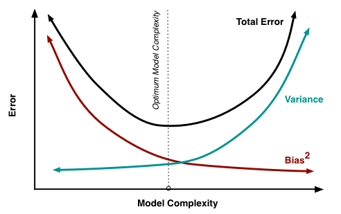
In machine learning bias-variance decomposition is also called bias-variance tradeoff:

Asymptotic normality

Estimation \(\widehat{\theta}_n\) is asymptotically normal if \(\frac{\widehat{\theta}_n - \theta}{\mathrm{se}(\widehat{\theta}_n)} \stackrel{D}{\to} \mathcal N(0,1)\), i.e.,

\[ \lim\limits_{n\to\infty}\mathbb P\bigg(\frac{\widehat{\theta}_n - \theta}{\mathrm{se}(\widehat{\theta}_n)} \leqslant z\bigg) = \mathbb \Phi(z), \quad \mathrm{se}(\widehat{\theta}_n) = \sqrt{\mathbb V\widehat{\theta}_n}. \]

If \(X_1, \ldots, X_n\) is an i.i.d. sample from some distribution with finite expection \(\mu\) and variance \(\sigma^2\), then according to the central limit theorem \(\overline X_n\) is asymptotically normal estimation of \(\mu\).

Maximum likelihood estimation (MLE)

Let i.i.d. sample \(X_1, \ldots, X_n \sim F_\theta(x)\). Правдоподобие (функция правдоподобия, likelihood) выборки \(X_1,\ldots, \ldots X_n\) — это просто её совместная pmf или pdf. Вне зависимости от типа распределения будем обозначать правдоподобие как

\[ \mathcal L(\theta) \equiv L(X_1, \ldots, X_n \vert \theta) = p(X_1, \ldots, X_n \vert \theta). \]

Если выборка i.i.d., то функция правдоподобия распадается в произведение одномерных функций:

\[ L(X_1, \ldots, X_n \vert \theta) = \prod\limits_{k=1}^n \log p(X_k\vert \theta). \]

Оценка максимального правдоподобия (maximum likelihood estimation, MLE) максимизирует правдоподобие:

\[ \widehat \theta_{\mathrm{ML}} = \arg \max\limits_{\theta} \mathcal L(\theta) \]

Поскольку максимизировать сумму проще, чем произведение, обычно переходят к логарифму правдоподобия (log-likelihood). Это особенно удобно в случае i.i.d. выборки, тогда

\[ \widehat \theta_{\mathrm{ML}} = \arg \max\limits_{\theta} \log \mathcal L(\theta) = \arg \max\limits_{\theta} \sum\limits_{k=1}^n p(X_k\vert \theta). \]

Properties of MLE

• consistency: \(\widehat \theta_{\mathrm{ML}} \stackrel{P}{\to} \theta\);

• equivariance: if \(\widehat \theta_{\mathrm{ML}}\) — MLE for \(\theta\) then \(\varphi(\theta)\) — MLE for \(\varphi(\theta)\);

• asymptotic normality: \(\frac{\widehat \theta_{\mathrm{ML}} - \theta}{\widehat{\mathrm{se}}} \stackrel{D}{\to} \mathcal N(0,1)\);

• асимптотическая оптимальность: при достаточно больших \(n\) оценка \(\widehat \theta_{\mathrm{ML}}\) имеет минимальную дисперсию.

Exercises

1. Let \(X_1, \ldots, X_n\) be an i.i.d. sample from \(U[0, \theta]\) and \(\widehat\theta = X_{(n)}\). Is this estimation unbiased? Asymptotically unbiased? Consistent?

2. Show that estimation \(\widehat{\theta}_n\) is consistent if it is asymptotically unbiased and \(\lim\limits_{n\to\infty}\mathbb{V}(\widehat{\theta}_n) = 0\).

3. Let \(X_1, \ldots, X_n\) be an i.i.d. sample from \(U[0, 2\theta]\). Show that sample median \(\mathrm{med}(X_1, \ldots, X_n)\) is unbiased estimation of \(\theta\).

4. Let \(X_1, \ldots, X_n\) be an i.i.d. sample from a distribution with finite moments \(\mathbb EX_1\) and \(\mathbb EX_1^2\). Is sample variance \(\overline S_n\) unbiased estimation of \(\theta = \mathbb V X_1\)? Asymptotically unbiased?

5. There are \(k\) heads and \(n-k\) tails in \(n\) independent Bernoulli trials. Find MLE of the probability of heads.

6. Find MLE estimation of \(\lambda\) if \(X_1, \ldots, X_n\) is an i.i.d. sample from \(\mathrm{Pois}(\lambda)\).

7. Let \(X_1, \ldots, X_n\) be i.i.d. sample from \(\mathcal N(\mu, \tau)\). Find MLE of \(\mu\) and \(\tau\).

8. Find MLE estimation of \(a\) and \(b\) if \(X_1, \ldots, X_n \sim U[a, b]\).