Probabilistic models for linear regression

Consider a regression problem with dataset \(\mathcal D = \{(\boldsymbol x_i, y_i)\}_{i=1}^n\), \(y_i\in\mathbb R\). The probabilistic model for the linear regression model assumes that

\[ y_i = \boldsymbol x_i^{\mathsf T} \boldsymbol w + \varepsilon_i, \]

where \(\varepsilon_i\) is some random noise.

Gaussian model

In this setting the random noise is gaussian: \(\varepsilon_i \sim \mathcal N (0, \sigma^2)\). Hence,

\[ p(y_i \vert \boldsymbol x_i, \boldsymbol w) = \mathcal N(y_i \vert \boldsymbol x_i^{\mathsf T} \boldsymbol w, \sigma^2) = \frac 1{\sqrt{2\pi} \sigma} \exp\Big(-\frac{(\boldsymbol x_i^{\mathsf T} \boldsymbol w - y_i)^2}{2\sigma^2}\Big). \]

Q. What is \(\mathbb E y_i\)? \(\mathbb V y_i\)?

A picture from ML Handbook:

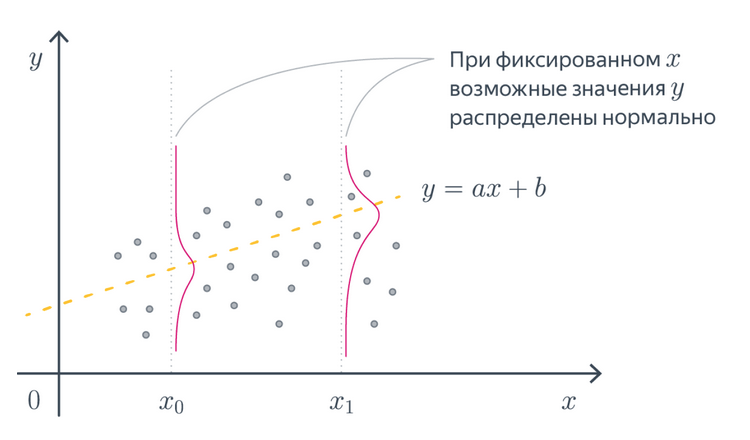
Q. What is \(\boldsymbol x_i\) and \(\boldsymbol w\) in this picture?

The likelihood of the dataset \(\mathcal D\) is

\[ p(\boldsymbol y \vert \boldsymbol X, \boldsymbol w) = \prod_{i=1}^n \mathcal N(y_i \vert\boldsymbol x_i^{\mathsf T} \boldsymbol w, \sigma^2) = \frac 1{(\sqrt{2\pi}\sigma)^n}\exp\Big(-\sum\limits_{i=1}^n \frac{(\boldsymbol x_i^{\mathsf T} \boldsymbol w - y_i)^2}{2\sigma^2}\Big). \]

Hence, the negative log-likelihood is

\[ \mathrm{NLL}(\boldsymbol w) = -\log p(\boldsymbol y \vert \boldsymbol X, \boldsymbol w)= \frac 1{2\sigma^2} \sum\limits_{i=1}^n (\boldsymbol x_i^{\mathsf T} \boldsymbol w - y_i)^2 + \frac n2\log(2\pi\sigma^2). \]

Q. How does this NLL relates to the loss function (19) of the linear regression model?

Thus, the optimal weights (21) of the linear regression with MSE loss coincide with MLE:

\[ \boldsymbol{\widehat w} = \arg\max\limits_{\boldsymbol w} p(\boldsymbol y \vert \boldsymbol X, \boldsymbol w) = \arg\min\limits_{\boldsymbol w} \mathrm{NLL}(\boldsymbol w). \]

Q. Let \(\sigma\) be also a learnable parameter. What is MLE \(\widehat \sigma^2\) for it?

Laplacian model

Now suppose that our loss function is MAE. Then

\[ \boldsymbol{\widehat w} = \arg\min\limits_{\boldsymbol w} \sum\limits_{i=1}^n \vert \boldsymbol x_i^{\mathsf T} \boldsymbol w - y_i\vert = \arg\max\limits_{\boldsymbol w} \Big(-\sum\limits_{i=1}^n \vert \boldsymbol x_i^{\mathsf T} \boldsymbol w - y_i\vert\Big) \]

Which probabilistic model will give

\[ \mathrm{NLL}(\boldsymbol w) = \frac 1b\sum\limits_{i=1}^n \vert \boldsymbol x_i^{\mathsf T} \boldsymbol w - y_i\vert + \mathrm{const}? \]

Well, then likelihood should be

\[ p(\boldsymbol y \vert \boldsymbol X, \boldsymbol w) \propto \exp\Big(-\frac 1b\sum\limits_{i=1}^n \vert\boldsymbol x_i^{\mathsf T} \boldsymbol w - y_i\vert\Big) = \prod\limits_{i=1}^n \exp\Big(-\frac{\vert\boldsymbol x_i^{\mathsf T} \boldsymbol w - y_i\vert} b\Big). \]

Hence,

\[ p(y_i \vert \boldsymbol x_i, \boldsymbol w) \propto \exp\Big(-\frac{\vert\boldsymbol x_i^{\mathsf T} \boldsymbol w - y_i\vert}b\Big), \]

and

\[ y_i \sim \mathrm{Laplace}(\boldsymbol x_i^{\mathsf T} \boldsymbol w, b). \]

Bayesian linear regression

Gaussian prior

Let prior distribution be Gaussian:

\[ p(\boldsymbol w) = \mathcal N(\boldsymbol 0, \tau^2\boldsymbol I). \]

Then posterior distribution

\[ p(\boldsymbol w \vert \boldsymbol X, \boldsymbol y) \propto p( \boldsymbol y \vert \boldsymbol X, \boldsymbol w)p(\boldsymbol w) \]

is also Gaussian.

Example

Let \(y = ax\) be 1-d linear regression model and \(p(a) = \mathcal N(0, \tau^2)\). Find posterior \(p(a \vert \boldsymbol x, \boldsymbol y)\) after observing a dataset \(\{(x_i, y_i)\}_{i=1}^n\).

Possible answer

\[ p(a \vert \boldsymbol x, \boldsymbol y) = \mathcal N\Bigg(\frac{\boldsymbol x^\mathsf{T}\boldsymbol y}{\frac{\sigma^2}{\tau^2}+ \sum\limits_{i=1}^n x_i^2}, \frac 1{\frac 1{\tau^2} + \frac 1{\sigma^2}\sum\limits_{i=1}^n x_i^2}\Bigg) \]

To find \(\boldsymbol {\widehat w}_{\mathrm{MAP}}\), we need to maximize posterior \(p(\boldsymbol w \vert \boldsymbol X, \boldsymbol y)\). This is the same as to minimize

\[ -\log p(\boldsymbol w \vert \boldsymbol X, \boldsymbol y) = -\log p( \boldsymbol y \vert \boldsymbol X, \boldsymbol w) - \log p(\boldsymbol w) + \mathrm{const}. \]

Recall that \(p( \boldsymbol y \vert \boldsymbol X, \boldsymbol w) = \mathcal N(\boldsymbol y \vert \boldsymbol{Xw}, \sigma^2 \boldsymbol I)\). According to calculations from ML Handbook

\[ -\log p( \boldsymbol y \vert \boldsymbol X, \boldsymbol w) - \log p(\boldsymbol w) = \frac 1{2\sigma^2} \sum\limits_{i=1}^n (y_i -\boldsymbol x_i^\mathsf{T} \boldsymbol w)^2 + \frac 1{2\tau^2} \sum\limits_{j=1}^d w_j^2 + \mathrm{const}. \]

Hence,

\[ \boldsymbol {\widehat w}_{\mathrm{MAP}} = \arg\min\limits_{\boldsymbol w} \bigg(\sum\limits_{i=1}^n (y_i -\boldsymbol x_i^\mathsf{T} \boldsymbol w)^2 + \frac{\sigma^2}{\tau^2} \Vert \boldsymbol w \Vert_2^2\bigg). \]

Can you recognize the objective of the ridge regression with \(C = \frac{\sigma^2}{\tau^2}\)? The analytical solution is

\[ \boldsymbol {\widehat w}_{\mathrm{MAP}} = \Big(\boldsymbol X^\mathsf{T} \boldsymbol X + \frac{\sigma^2}{\tau^2}\boldsymbol I\Big)^{-1}\boldsymbol X^{\mathsf{T}}\boldsymbol y. \]

Contnuing calculations, we can find posterior:

\[ p(\boldsymbol w \vert \boldsymbol X, \boldsymbol y) = \mathcal N\Big(\boldsymbol {\widehat w}_{\mathrm{MAP}},\Big(\frac 1{\sigma^2}\boldsymbol X^\mathsf{T} \boldsymbol X + \frac{1}{\tau^2}\boldsymbol I\Big)^{-1} \Big). \]

Laplacian prior

Consinder the following prior: \(w_1, \ldots, w_d\) are i.i.d laplacian random variables with parameter \(\lambda\). Then

\[ p(\boldsymbol w) = \prod\limits_{j=1}^d \mathrm{Laplace}(w_j \vert \lambda) = \prod\limits_{j=1}^d \frac\lambda 2e^{-\lambda|w_j|} = \frac {\lambda^d}{2^d} \exp\Big(-\sum\limits_{j=1}^d\lambda|w_j|\Big). \]

The likelihood \(p( \boldsymbol y \vert \boldsymbol X, \boldsymbol w)\) is still \(\mathcal N(\boldsymbol{Xw}, \sigma^2 \boldsymbol I)\). Then

\[ -\log p(\boldsymbol w \vert \boldsymbol X, \boldsymbol y) = \frac 1{2\sigma^2} \sum\limits_{i=1}^n (y_i -\boldsymbol x_i^{\mathsf{T}} \boldsymbol w)^2 + \lambda\sum\limits_{j=1}^d \vert w_j\vert + \mathrm{const}. \]

Hence, maximum a posteriori estimation is

\[ \boldsymbol {\widehat w}_{\mathrm{MAP}} = \arg\min\limits_{\boldsymbol w} \Big(\Vert \boldsymbol{Xw} - \boldsymbol y\Vert_2^2 + 2\sigma^2 \lambda \Vert \boldsymbol w \Vert_1\Big). \]

This is exactly the objective of LASSO.