HW3

Deadline: 24.11.2024 23:59 (GMT+5)

Task 3.1 (2 points)

Let \(x_1, \dots, x_n \sim U[0,1]\). Sort them in the nondecreasing order:

\[ x_{(1)} \leqslant x_{(2)} \leqslant \ldots \leqslant x_{(k)} \leqslant\ldots\leqslant x_{(n)}. \]

The \(k\)-th element \(x_{(k)}\) in this sequence is called \(k\)-th order statistics. Show that \(x_{(k)} \sim \mathrm{Beta}(k, n+1 -k)\). Do it in two ways:

• experimentally: generate a random matrix of shape \(N \times n\) (try \(N = 1000, 10000, 100000\)), calculate \(k\)-th order statistics for each row and plot historgram of these values along with pdf of beta distribution. (1 point)

• theoretically: present a mathematical proof of this statement (1 point)

Warning

To get full points for the experimental part you should avoid pythonic loops when generating random matrix. The only place where for loop is allowed is iterating over several values of \(N\).

YOUR SOLUTION HERE

Your historgram for a paticular value of \(N\) should look like this:

from scipy.stats import beta, gamma
import numpy as np
import matplotlib.pyplot as plt

%config InlineBackend.figure_formats = ['svg']

def beta_hist(a, b, N=10000):
    xs = np.linspace(0.001, 0.999, num=1000)
    plt.hist(beta(a, b).rvs(size=N), bins=100, color='b', density=True)
    plt.plot(xs, beta(a, b).pdf(xs), c='r', lw=2, ls="--")
    plt.grid(ls=":")
    
beta_hist(3, 5)

Task 3.2 (2 points)

• Find KL divergence between \(p\sim \mathrm{Geom}(s)\) and \(q\sim \mathrm{Geom}(t)\), \(0 < s, t < 1\). Is \(\mathbb{KL}(p, q) = 0\) when \(s = t\)? Does equality \(\mathbb{KL}(p, q) = \mathbb{KL}(q, p)\) hold? (1.5 points)

• Plot the graphs of \(\mathbb{KL}(p, q)\) as functions of \(s\) for several fixed values of \(t\). (0.5 points)

YOUR SOLUTION HERE

Task 3.3 (2 points)

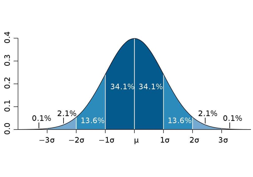
For a one-dimensional gaussian \(\xi \sim \mathcal N(\mu, \sigma^2)\) there are well-known rules of one, two and three sigmas:

• one-sigma rule: \(\mathbb P(\vert \xi - \mu \vert \leqslant \sigma) = \Phi(1) - \Phi(-1) \approx 0.6827\)

• two-sigma rule: \(\mathbb P(\vert \xi - \mu \vert \leqslant 2\sigma) = \Phi(2) - \Phi(-2) \approx 0.9545\)

• three-sigma rule: \(\mathbb P(\vert \xi - \mu \vert \leqslant 3\sigma) = \Phi(3) - \Phi(-3) \approx 0.9973\)

from scipy.stats import norm

norm.cdf(1) - norm.cdf(-1), norm.cdf(2) - norm.cdf(-2), norm.cdf(3) - norm.cdf(-3)

(np.float64(0.6826894921370859),
 np.float64(0.9544997361036416),
 np.float64(0.9973002039367398))

Compute analagous values for a 2-d gaussian distribution \(\boldsymbol \xi \sim \mathcal N(\boldsymbol 0, \boldsymbol I_2)\). Namely, find \(\mathbb P(\Vert\boldsymbol \xi\Vert_2 \leqslant 1)\), \(\mathbb P(\Vert\boldsymbol \xi\Vert_2 \leqslant 2)\), \(\mathbb P(\Vert\boldsymbol \xi\Vert_2 \leqslant 3)\)

• analytically (1 point)

• numerically, using scipy or Monte Carlo methods (1 point)

YOUR SOLUTION HERE

Task 3.4 (1 point)

Let \(X_1, \ldots, X_n\) is an i.i.d. sample form \(U[0, 2\theta]\). The parameter \(\theta\) can be estimated as \(\widehat\theta = \overline X_n\) (sample average) or \(\tilde\theta = \mathrm{med}(X_1, \ldots, X_n)\) (sample median). According to ML Handbook, both estimations are unbiased, and \(\mathbb V \widehat\theta = \frac{\theta^2}{3n}\), \(\mathbb V \tilde\theta = \frac{\theta^2}{n+3}\). Hence, due to the central limit theorem

\[ \widehat\theta \approx \mathcal N\Big(\theta, \frac{\theta^2}{3n}\Big), \quad \tilde\theta \approx \mathcal N\Big(\theta, \frac{\theta^2}{n+3}\Big), \quad n \gg 1. \]

Plot two histograms on the same plot verifying this theoretical statements. Add two dashed lines for gaussians as it done here. Try different values of \(n\): \(100\), \(1000\), \(10^4\), \(10^5\).