Classification and regression trees

See also

A decision tree chapter in ML Handbook

Binary splitting

Suppose we have a dataset $\mathcal{D}=(\mathit{X},\mathit{y})$ with $n$ training samples, each of which has $d$ numeric features. To make a binary split one needs to do the following:

• take $j$-th feature, $1⩽j⩽d$

• select a threshold $t$

• split dataset by condition ${\mathit{X}}_{:,j}⩽t$

After that the dataset $\mathcal{D}$ has been split into two parts, ${\mathcal{D}}_{\ell }$ and ${\mathcal{D}}_r$, such that $j$-th feature of samples from ${\mathcal{D}}_{\ell }$ is greater than $t$ whereas $j$-th feature of samples from ${\mathcal{D}}_r$ is does not exceed $t$.

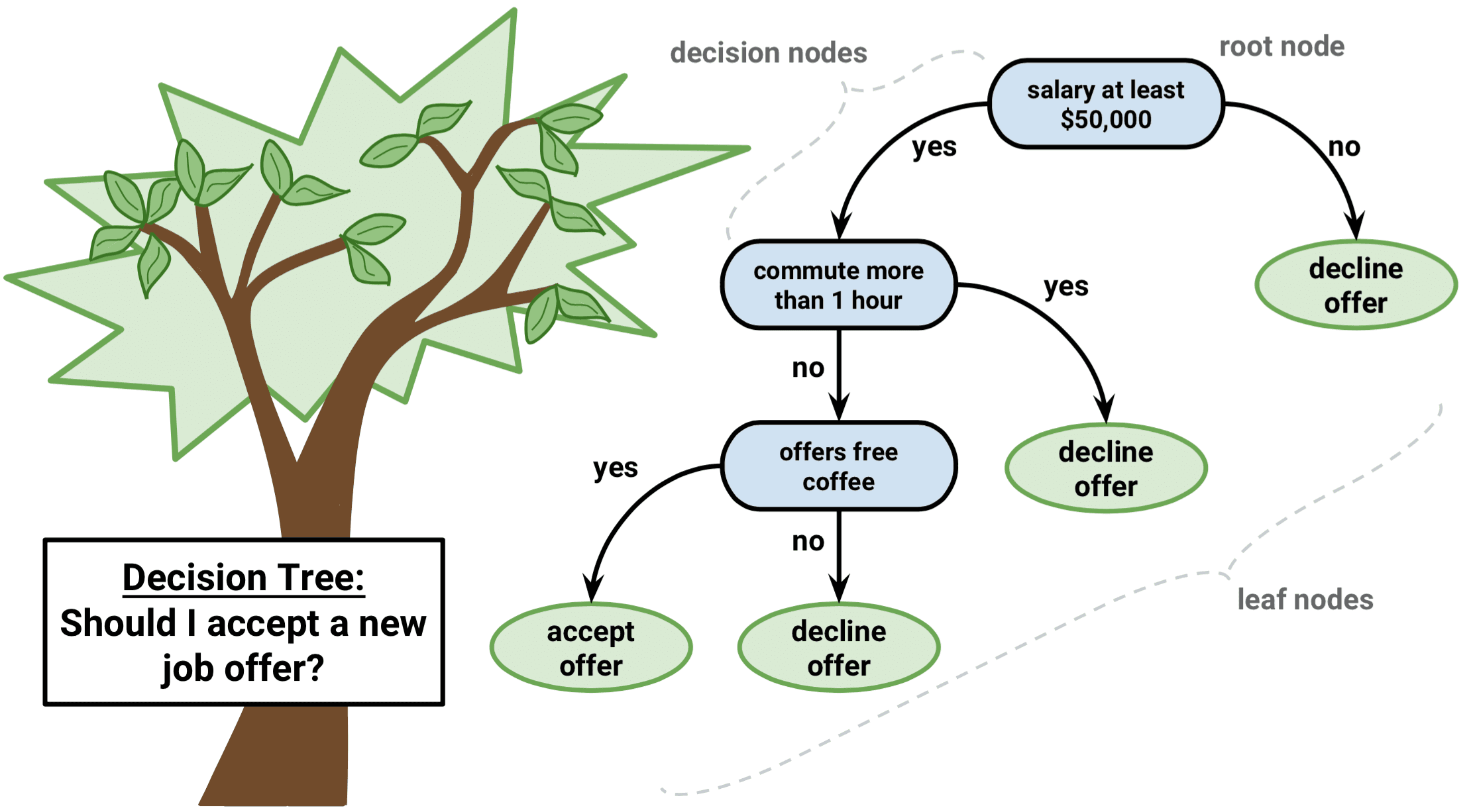
This splitting operation continues recursively: apply binary splitting to both left and right nodes with datasets ${\mathcal{D}}_{\ell }$ and ${\mathcal{D}}_r$ respectively. On this way we obtain a binary decision tree which consists of decision nodes.

Q. How many variants are there for selection a feature $j$ and a threshold $t$ on the first step when we create the root node? Suppose that we want to avoid trivial splits when one of subnodes is empty.

Stopping criteria

Where should we stop and not do split a decision node anymore? There could be different stategies.

• All data points in a node belong to the same class (for classification)

• A pre-defined depth of the tree is reached

• A pre-defined minimum leaf size is reached

• Further splitting doesn’t add much value

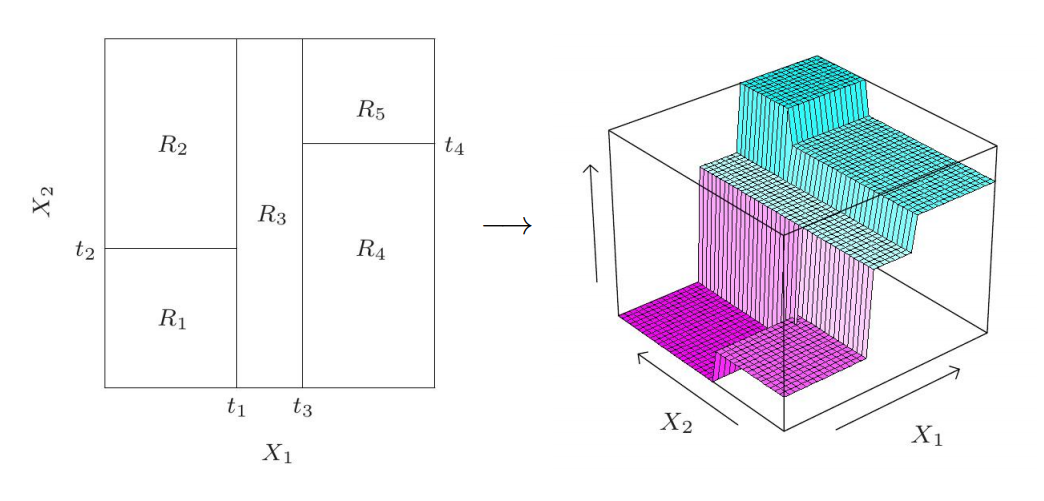
If a node is not split, it becomes a leaf. Each leaf produces a prediction as majority class of samples in this leaf (for classification) or average of targets (for regression). A regression tree is always a piecewise constant model.

Iris dataset

This is an example from sklearn.

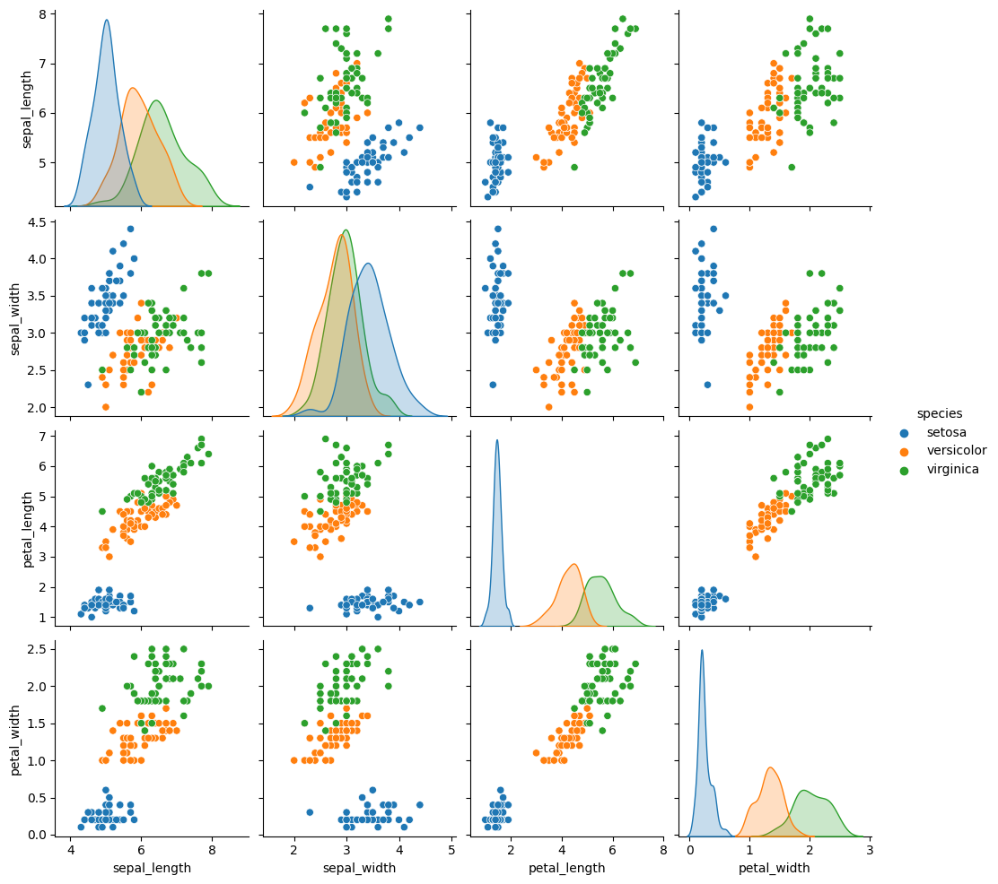
Download and visualize Iris dataset:

import seaborn as sns
iris = sns.load_dataset("iris")
sns.pairplot(iris, hue="species");

Fit decision tree classifier:

from sklearn import tree

y = iris['species']
X = iris.drop("species", axis=1)
clf = tree.DecisionTreeClassifier()
clf = clf.fit(X, y)
print("Accuracy:", clf.score(X, y))

Accuracy: 1.0

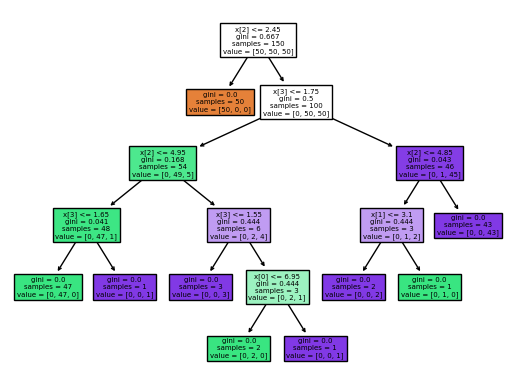
Plot the tree:

tree.plot_tree(clf, filled=True);

A prettier tree can be drawn by graphviz:

import graphviz

dot_data = tree.export_graphviz(clf, out_file=None, 
                     feature_names=iris.columns[:-1],  
                     class_names=['setosa', 'versicolor', 'virginica'],  
                     filled=True, rounded=True,  
                     special_characters=True)  
graph = graphviz.Source(dot_data)  
graph 

To reduce overfitting, tree depth is usually limited. Depth $2$ is enough for this toy dataset:

clf = tree.DecisionTreeClassifier(max_depth=2)
clf = clf.fit(X, y)
print("Accuracy:", clf.score(X, y))

Accuracy: 0.96

MNIST

import numpy as np
import matplotlib.pyplot as plt
import seaborn as sns
from sklearn.metrics import accuracy_score, confusion_matrix
from sklearn.datasets import fetch_openml
from sklearn.model_selection import train_test_split

%config InlineBackend.figure_format = 'svg'

X, Y = fetch_openml('mnist_784', return_X_y=True, parser='auto')

X = X.astype(float).values / 255
Y = Y.astype(int).values

Visualize data:

Split into train and test:

X_train, X_test, y_train, y_test = train_test_split(X, Y, test_size=10000)
X_train.shape, X_test.shape, y_train.shape, y_test.shape

((60000, 784), (10000, 784), (60000,), (10000,))

Fit a decision tree model:

from sklearn.tree import DecisionTreeClassifier

DT = DecisionTreeClassifier()
DT.fit(X_train, y_train)

DecisionTreeClassifier()

In a Jupyter environment, please rerun this cell to show the HTML representation or trust the notebook.
On GitHub, the HTML representation is unable to render, please try loading this page with nbviewer.org.

Accuracy score:

print("Train accuracy:", DT.score(X_train, y_train))
print("Test accuracy:", DT.score(X_test, y_test))

Train accuracy: 1.0
Test accuracy: 0.8735

plt.figure(figsize=(10, 8))
plt.title("Decision tree on MNIST")
sns.heatmap(confusion_matrix(y_test, DT.predict(X_test)), annot=True);

Limit the tree depth and size of leaves:

DT = DecisionTreeClassifier(max_depth=15, min_samples_leaf=3)
DT.fit(X_train, y_train)

DecisionTreeClassifier(max_depth=15, min_samples_leaf=3)

In a Jupyter environment, please rerun this cell to show the HTML representation or trust the notebook.
On GitHub, the HTML representation is unable to render, please try loading this page with nbviewer.org.

print("Train accuracy:", DT.score(X_train, y_train))
print("Test accuracy:", DT.score(X_test, y_test))

Train accuracy: 0.9615166666666667
Test accuracy: 0.8776